Note

Go to the end to download the full example code. or to run this example in your browser via JupyterLite or Binder

Imputing missing values before building an estimator#

Missing values can be replaced by the mean, the median or the most frequent value using the basic SimpleImputer.

In this example we will investigate different imputation techniques:

imputation by the constant value 0
imputation by the mean value of each feature combined with a missing-ness indicator auxiliary variable
k nearest neighbor imputation
iterative imputation

We will use two datasets: Diabetes dataset which consists of 10 feature variables collected from diabetes patients with an aim to predict disease progression and California Housing dataset for which the target is the median house value for California districts.

As neither of these datasets have missing values, we will remove some values to create new versions with artificially missing data. The performance of RandomForestRegressor on the full original dataset is then compared the performance on the altered datasets with the artificially missing values imputed using different techniques.

# Authors: The scikit-learn developers
# SPDX-License-Identifier: BSD-3-Clause

Download the data and make missing values sets#

First we download the two datasets. Diabetes dataset is shipped with scikit-learn. It has 442 entries, each with 10 features. California Housing dataset is much larger with 20640 entries and 8 features. It needs to be downloaded. We will only use the first 400 entries for the sake of speeding up the calculations but feel free to use the whole dataset.

import numpy as np

from sklearn.datasets import fetch_california_housing, load_diabetes

rng = np.random.RandomState(42)

X_diabetes, y_diabetes = load_diabetes(return_X_y=True)
X_california, y_california = fetch_california_housing(return_X_y=True)
X_california = X_california[:300]
y_california = y_california[:300]
X_diabetes = X_diabetes[:300]
y_diabetes = y_diabetes[:300]


def add_missing_values(X_full, y_full):
    n_samples, n_features = X_full.shape

    # Add missing values in 75% of the lines
    missing_rate = 0.75
    n_missing_samples = int(n_samples * missing_rate)

    missing_samples = np.zeros(n_samples, dtype=bool)
    missing_samples[:n_missing_samples] = True

    rng.shuffle(missing_samples)
    missing_features = rng.randint(0, n_features, n_missing_samples)
    X_missing = X_full.copy()
    X_missing[missing_samples, missing_features] = np.nan
    y_missing = y_full.copy()

    return X_missing, y_missing


X_miss_california, y_miss_california = add_missing_values(X_california, y_california)

X_miss_diabetes, y_miss_diabetes = add_missing_values(X_diabetes, y_diabetes)

Impute the missing data and score#

Now we will write a function which will score the results on the differently imputed data. Let’s look at each imputer separately:

rng = np.random.RandomState(0)

from sklearn.ensemble import RandomForestRegressor

# To use the experimental IterativeImputer, we need to explicitly ask for it:
from sklearn.experimental import enable_iterative_imputer  # noqa
from sklearn.impute import IterativeImputer, KNNImputer, SimpleImputer
from sklearn.model_selection import cross_val_score
from sklearn.pipeline import make_pipeline

N_SPLITS = 4
regressor = RandomForestRegressor(random_state=0)

Missing information#

In addition to imputing the missing values, the imputers have an add_indicator parameter that marks the values that were missing, which might carry some information.

def get_scores_for_imputer(imputer, X_missing, y_missing):
    estimator = make_pipeline(imputer, regressor)
    impute_scores = cross_val_score(
        estimator, X_missing, y_missing, scoring="neg_mean_squared_error", cv=N_SPLITS
    )
    return impute_scores


x_labels = []

mses_california = np.zeros(5)
stds_california = np.zeros(5)
mses_diabetes = np.zeros(5)
stds_diabetes = np.zeros(5)

Estimate the score#

First, we want to estimate the score on the original data:

def get_full_score(X_full, y_full):
    full_scores = cross_val_score(
        regressor, X_full, y_full, scoring="neg_mean_squared_error", cv=N_SPLITS
    )
    return full_scores.mean(), full_scores.std()


mses_california[0], stds_california[0] = get_full_score(X_california, y_california)
mses_diabetes[0], stds_diabetes[0] = get_full_score(X_diabetes, y_diabetes)
x_labels.append("Full data")

Replace missing values by 0#

Now we will estimate the score on the data where the missing values are replaced by 0:

def get_impute_zero_score(X_missing, y_missing):
    imputer = SimpleImputer(
        missing_values=np.nan, add_indicator=True, strategy="constant", fill_value=0
    )
    zero_impute_scores = get_scores_for_imputer(imputer, X_missing, y_missing)
    return zero_impute_scores.mean(), zero_impute_scores.std()


mses_california[1], stds_california[1] = get_impute_zero_score(
    X_miss_california, y_miss_california
)
mses_diabetes[1], stds_diabetes[1] = get_impute_zero_score(
    X_miss_diabetes, y_miss_diabetes
)
x_labels.append("Zero imputation")

kNN-imputation of the missing values#

KNNImputer imputes missing values using the weighted or unweighted mean of the desired number of nearest neighbors.

def get_impute_knn_score(X_missing, y_missing):
    imputer = KNNImputer(missing_values=np.nan, add_indicator=True)
    knn_impute_scores = get_scores_for_imputer(imputer, X_missing, y_missing)
    return knn_impute_scores.mean(), knn_impute_scores.std()


mses_california[2], stds_california[2] = get_impute_knn_score(
    X_miss_california, y_miss_california
)
mses_diabetes[2], stds_diabetes[2] = get_impute_knn_score(
    X_miss_diabetes, y_miss_diabetes
)
x_labels.append("KNN Imputation")

Impute missing values with mean#

def get_impute_mean(X_missing, y_missing):
    imputer = SimpleImputer(missing_values=np.nan, strategy="mean", add_indicator=True)
    mean_impute_scores = get_scores_for_imputer(imputer, X_missing, y_missing)
    return mean_impute_scores.mean(), mean_impute_scores.std()


mses_california[3], stds_california[3] = get_impute_mean(
    X_miss_california, y_miss_california
)
mses_diabetes[3], stds_diabetes[3] = get_impute_mean(X_miss_diabetes, y_miss_diabetes)
x_labels.append("Mean Imputation")

Iterative imputation of the missing values#

Another option is the IterativeImputer. This uses round-robin linear regression, modeling each feature with missing values as a function of other features, in turn. The version implemented assumes Gaussian (output) variables. If your features are obviously non-normal, consider transforming them to look more normal to potentially improve performance.

def get_impute_iterative(X_missing, y_missing):
    imputer = IterativeImputer(
        missing_values=np.nan,
        add_indicator=True,
        random_state=0,
        n_nearest_features=3,
        max_iter=1,
        sample_posterior=True,
    )
    iterative_impute_scores = get_scores_for_imputer(imputer, X_missing, y_missing)
    return iterative_impute_scores.mean(), iterative_impute_scores.std()


mses_california[4], stds_california[4] = get_impute_iterative(
    X_miss_california, y_miss_california
)
mses_diabetes[4], stds_diabetes[4] = get_impute_iterative(
    X_miss_diabetes, y_miss_diabetes
)
x_labels.append("Iterative Imputation")

mses_diabetes = mses_diabetes * -1
mses_california = mses_california * -1

Plot the results#

Finally we are going to visualize the score:

import matplotlib.pyplot as plt

n_bars = len(mses_diabetes)
xval = np.arange(n_bars)

colors = ["r", "g", "b", "orange", "black"]

# plot diabetes results
plt.figure(figsize=(12, 6))
ax1 = plt.subplot(121)
for j in xval:
    ax1.barh(
        j,
        mses_diabetes[j],
        xerr=stds_diabetes[j],
        color=colors[j],
        alpha=0.6,
        align="center",
    )

ax1.set_title("Imputation Techniques with Diabetes Data")
ax1.set_xlim(left=np.min(mses_diabetes) * 0.9, right=np.max(mses_diabetes) * 1.1)
ax1.set_yticks(xval)
ax1.set_xlabel("MSE")
ax1.invert_yaxis()
ax1.set_yticklabels(x_labels)

# plot california dataset results
ax2 = plt.subplot(122)
for j in xval:
    ax2.barh(
        j,
        mses_california[j],
        xerr=stds_california[j],
        color=colors[j],
        alpha=0.6,
        align="center",
    )

ax2.set_title("Imputation Techniques with California Data")
ax2.set_yticks(xval)
ax2.set_xlabel("MSE")
ax2.invert_yaxis()
ax2.set_yticklabels([""] * n_bars)

plt.show()

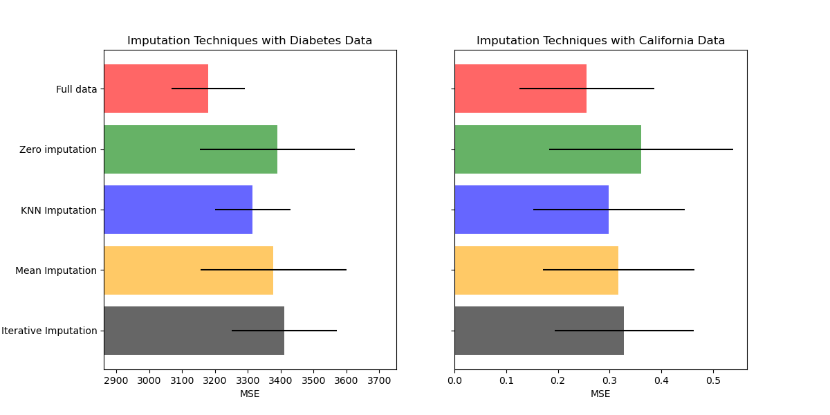
Imputation Techniques with Diabetes Data, Imputation Techniques with California Data

You can also try different techniques. For instance, the median is a more robust estimator for data with high magnitude variables which could dominate results (otherwise known as a ‘long tail’).

Total running time of the script: (0 minutes 11.411 seconds)