1.16. Probability calibration#
When performing classification you often want not only to predict the class
label, but also obtain a probability of the respective label. This probability
gives you some kind of confidence on the prediction. Some models can give you
poor estimates of the class probabilities and some even do not support
probability prediction (e.g., some instances of
SGDClassifier).
The calibration module allows you to better calibrate
the probabilities of a given model, or to add support for probability
prediction.
Well calibrated classifiers are probabilistic classifiers for which the output of the predict_proba method can be directly interpreted as a confidence level. For instance, a well calibrated (binary) classifier should classify the samples such that among the samples to which it gave a predict_proba value close to, say, 0.8, approximately 80% actually belong to the positive class.
Before we show how to re-calibrate a classifier, we first need a way to detect how good a classifier is calibrated.
Note
Strictly proper scoring rules for probabilistic predictions like
sklearn.metrics.brier_score_loss and
sklearn.metrics.log_loss assess calibration (reliability) and
discriminative power (resolution) of a model, as well as the randomness of the data
(uncertainty) at the same time. This follows from the well-known Brier score
decomposition of Murphy [1]. As it is not clear which term dominates, the score is
of limited use for assessing calibration alone (unless one computes each term of
the decomposition). A lower Brier loss, for instance, does not necessarily
mean a better calibrated model, it could also mean a worse calibrated model with much
more discriminatory power, e.g. using many more features.
1.16.1. Calibration curves#
Calibration curves, also referred to as reliability diagrams (Wilks 1995 [2]), compare how well the probabilistic predictions of a binary classifier are calibrated. It plots the frequency of the positive label (to be more precise, an estimation of the conditional event probability \(P(Y=1|\text{predict_proba})\)) on the y-axis against the predicted probability predict_proba of a model on the x-axis. The tricky part is to get values for the y-axis. In scikit-learn, this is accomplished by binning the predictions such that the x-axis represents the average predicted probability in each bin. The y-axis is then the fraction of positives given the predictions of that bin, i.e. the proportion of samples whose class is the positive class (in each bin).
The top calibration curve plot is created with
CalibrationDisplay.from_estimator, which uses calibration_curve to
calculate the per bin average predicted probabilities and fraction of positives.
CalibrationDisplay.from_estimator
takes as input a fitted classifier, which is used to calculate the predicted
probabilities. The classifier thus must have predict_proba method. For
the few classifiers that do not have a predict_proba method, it is
possible to use CalibratedClassifierCV to calibrate the classifier
outputs to probabilities.
The bottom histogram gives some insight into the behavior of each classifier by showing the number of samples in each predicted probability bin.
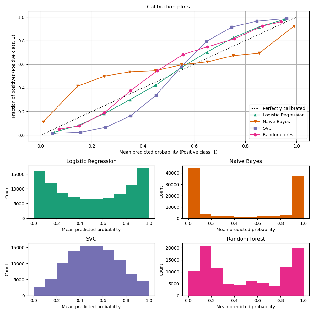
LogisticRegression is more likely to return well calibrated predictions by itself as it has a
canonical link function for its loss, i.e. the logit-link for the Log loss.
In the unpenalized case, this leads to the so-called balance property, see [8] and Logistic regression.
In the plot above, data is generated according to a linear mechanism, which is
consistent with the LogisticRegression model (the model is ‘well specified’),
and the value of the regularization parameter C is tuned to be
appropriate (neither too strong nor too low). As a consequence, this model returns
accurate predictions from its predict_proba method.
In contrast to that, the other shown models return biased probabilities; with
different biases per model.
GaussianNB (Naive Bayes) tends to push probabilities to 0 or 1 (note the counts
in the histograms). This is mainly because it makes the assumption that
features are conditionally independent given the class, which is not the
case in this dataset which contains 2 redundant features.
RandomForestClassifier shows the opposite behavior: the histograms
show peaks at probabilities approximately 0.2 and 0.9, while probabilities
close to 0 or 1 are very rare. An explanation for this is given by
Niculescu-Mizil and Caruana [3]: “Methods such as bagging and random
forests that average predictions from a base set of models can have
difficulty making predictions near 0 and 1 because variance in the
underlying base models will bias predictions that should be near zero or one
away from these values. Because predictions are restricted to the interval
[0,1], errors caused by variance tend to be one-sided near zero and one. For
example, if a model should predict \(p = 0\) for a case, the only way bagging
can achieve this is if all bagged trees predict zero. If we add noise to the
trees that bagging is averaging over, this noise will cause some trees to
predict values larger than 0 for this case, thus moving the average
prediction of the bagged ensemble away from 0. We observe this effect most
strongly with random forests because the base-level trees trained with
random forests have relatively high variance due to feature subsetting.” As
a result, the calibration curve shows a characteristic sigmoid shape, indicating that
the classifier could trust its “intuition” more and return probabilities closer
to 0 or 1 typically.
LinearSVC (SVC) shows an even more sigmoid curve than the random forest, which
is typical for maximum-margin methods (compare Niculescu-Mizil and Caruana [3]), which
focus on difficult to classify samples that are close to the decision boundary (the
support vectors).
1.16.2. Calibrating a classifier#
Calibrating a classifier consists of fitting a regressor (called a calibrator) that maps the output of the classifier (as given by decision_function or predict_proba) to a calibrated probability in [0, 1]. Denoting the output of the classifier for a given sample by \(f_i\), the calibrator tries to predict the conditional event probability \(P(y_i = 1 | f_i)\).
Ideally, the calibrator is fit on a dataset independent of the training data used to fit the classifier in the first place. This is because performance of the classifier on its training data would be better than for novel data. Using the classifier output of training data to fit the calibrator would thus result in a biased calibrator that maps to probabilities closer to 0 and 1 than it should.
1.16.3. Usage#
The CalibratedClassifierCV class is used to calibrate a classifier.
CalibratedClassifierCV uses a cross-validation approach to ensure
unbiased data is always used to fit the calibrator. The data is split into \(k\)
(train_set, test_set) couples (as determined by cv). When ensemble=True
(default), the following procedure is repeated independently for each
cross-validation split:
a clone of
base_estimatoris trained on the train subsetthe trained
base_estimatormakes predictions on the test subsetthe predictions are used to fit a calibrator (either a sigmoid or isotonic regressor) (when the data is multiclass, a calibrator is fit for every class)
This results in an
ensemble of \(k\) (classifier, calibrator) couples where each calibrator maps
the output of its corresponding classifier into [0, 1]. Each couple is exposed
in the calibrated_classifiers_ attribute, where each entry is a calibrated
classifier with a predict_proba method that outputs calibrated
probabilities. The output of predict_proba for the main
CalibratedClassifierCV instance corresponds to the average of the
predicted probabilities of the \(k\) estimators in the calibrated_classifiers_
list. The output of predict is the class that has the highest
probability.
It is important to choose cv carefully when using ensemble=True.
All classes should be present in both train and test subsets for every split.
When a class is absent in the train subset, the predicted probability for that
class will default to 0 for the (classifier, calibrator) couple of that split.
This skews the predict_proba as it averages across all couples.
When a class is absent in the test subset, the calibrator for that class
(within the (classifier, calibrator) couple of that split) is
fit on data with no positive class. This results in ineffective calibration.
When ensemble=False, cross-validation is used to obtain ‘unbiased’
predictions for all the data, via
cross_val_predict.
These unbiased predictions are then used to train the calibrator. The attribute
calibrated_classifiers_ consists of only one (classifier, calibrator)
couple where the classifier is the base_estimator trained on all the data.
In this case the output of predict_proba for
CalibratedClassifierCV is the predicted probabilities obtained
from the single (classifier, calibrator) couple.
The main advantage of ensemble=True is to benefit from the traditional
ensembling effect (similar to Bagging meta-estimator). The resulting ensemble should
both be well calibrated and slightly more accurate than with ensemble=False.
The main advantage of using ensemble=False is computational: it reduces the
overall fit time by training only a single base classifier and calibrator
pair, decreases the final model size and increases prediction speed.
Alternatively an already fitted classifier can be calibrated by using a
FrozenEstimator as
CalibratedClassifierCV(estimator=FrozenEstimator(estimator)).
It is up to the user to make sure that the data used for fitting the classifier
is disjoint from the data used for fitting the regressor.
CalibratedClassifierCV supports the use of two regression techniques
for calibration via the method parameter: "sigmoid" and "isotonic".
1.16.3.1. Sigmoid#
The sigmoid regressor, method="sigmoid" is based on Platt’s logistic model [4]:
where \(y_i\) is the true label of sample \(i\) and \(f_i\) is the output of the un-calibrated classifier for sample \(i\). \(A\) and \(B\) are real numbers to be determined when fitting the regressor via maximum likelihood.
The sigmoid method assumes the calibration curve can be corrected by applying a sigmoid function to the raw predictions. This assumption has been empirically justified in the case of Support Vector Machines with common kernel functions on various benchmark datasets in section 2.1 of Platt 1999 [4] but does not necessarily hold in general. Additionally, the logistic model works best if the calibration error is symmetrical, meaning the classifier output for each binary class is normally distributed with the same variance [7]. This can be a problem for highly imbalanced classification problems, where outputs do not have equal variance.
In general this method is most effective for small sample sizes or when the un-calibrated model is under-confident and has similar calibration errors for both high and low outputs.
1.16.3.2. Isotonic#
The method="isotonic" fits a non-parametric isotonic regressor, which outputs
a step-wise non-decreasing function, see sklearn.isotonic. It minimizes:
subject to \(\hat{f}_i \geq \hat{f}_j\) whenever
\(f_i \geq f_j\). \(y_i\) is the true
label of sample \(i\) and \(\hat{f}_i\) is the output of the
calibrated classifier for sample \(i\) (i.e., the calibrated probability).
This method is more general when compared to 'sigmoid' as the only restriction
is that the mapping function is monotonically increasing. It is thus more
powerful as it can correct any monotonic distortion of the un-calibrated model.
However, it is more prone to overfitting, especially on small datasets [6].
Overall, 'isotonic' will perform as well as or better than 'sigmoid' when
there is enough data (greater than ~ 1000 samples) to avoid overfitting [3].
Note
Impact on ranking metrics like AUC
It is generally expected that calibration does not affect ranking metrics such as
ROC-AUC. However, these metrics might differ after calibration when using
method="isotonic" since isotonic regression introduces ties in the predicted
probabilities. This can be seen as within the uncertainty of the model predictions.
In case, you strictly want to keep the ranking and thus AUC scores, use
method="sigmoid" which is a strictly monotonic transformation and thus keeps
the ranking.
1.16.3.3. Multiclass support#
Both isotonic and sigmoid regressors only
support 1-dimensional data (e.g., binary classification output) but are
extended for multiclass classification if the base_estimator supports
multiclass predictions. For multiclass predictions,
CalibratedClassifierCV calibrates for
each class separately in a OneVsRestClassifier fashion [5]. When
predicting
probabilities, the calibrated probabilities for each class
are predicted separately. As those probabilities do not necessarily sum to
one, a postprocessing is performed to normalize them.
On the other hand, temperature scaling naturally supports multiclass predictions by working with logits and finally applying the softmax function.
1.16.3.4. Temperature Scaling#
For a multi-class classification problem with \(n\) classes, temperature scaling
[9], method="temperature", produces class probabilities by modifying the softmax
function with a temperature parameter \(T\):
where, for a given sample, \(z\) is the vector of logits for each class as predicted by the estimator to be calibrated. In terms of scikit-learn’s API, this corresponds to the output of decision_function or to the logarithm of predict_proba. Probabilities are converted to logits by first adding a tiny positive constant to avoid numerical issues with logarithm of zero, and then applying the natural logarithm.
The parameter \(T\) is learned by minimizing log_loss,
i.e. cross-entropy loss, on a hold-out (calibration) set. Note that \(T\) does not
affect the location of the maximum in the softmax output. Therefore, temperature scaling
does not alter the accuracy of the calibrating estimator.
The main advantage of temperature scaling over other calibration methods is that it provides a natural way to obtain (better) calibrated multi-class probabilities with just one free parameter in contrast to using a “One-vs-Rest” scheme that adds more parameters for each single class.
Examples
References