1.10. Decision Trees#
Decision Trees (DTs) are a non-parametric supervised learning method used for classification and regression. The goal is to create a model that predicts the value of a target variable by learning simple decision rules inferred from the data features. A tree can be seen as a piecewise constant approximation.
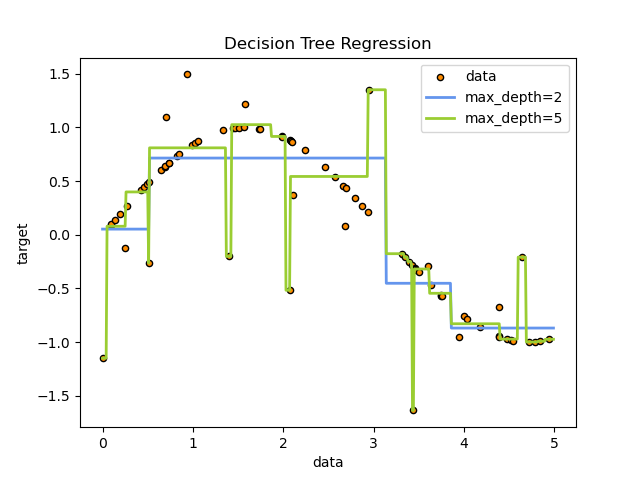
For instance, in the example below, decision trees learn from data to approximate a sine curve with a set of if-then-else decision rules. The deeper the tree, the more complex the decision rules and the fitter the model.
Some advantages of decision trees are:
Simple to understand and to interpret. Trees can be visualized.
Requires little data preparation. Other techniques often require data normalization, dummy variables need to be created and blank values to be removed. Some tree and algorithm combinations support missing values.
The cost of using the tree (i.e., predicting data) is logarithmic in the number of data points used to train the tree.
Able to handle both numerical and categorical data. However, the scikit-learn implementation does not support categorical variables for now. Other techniques are usually specialized in analyzing datasets that have only one type of variable. See algorithms for more information.
Able to handle multi-output problems.
Uses a white box model. If a given situation is observable in a model, the explanation for the condition is easily explained by boolean logic. By contrast, in a black box model (e.g., in an artificial neural network), results may be more difficult to interpret.
Possible to validate a model using statistical tests. That makes it possible to account for the reliability of the model.
Performs well even if its assumptions are somewhat violated by the true model from which the data were generated.
The disadvantages of decision trees include:
Decision-tree learners can create over-complex trees that do not generalize the data well. This is called overfitting. Mechanisms such as pruning, setting the minimum number of samples required at a leaf node or setting the maximum depth of the tree are necessary to avoid this problem.
Decision trees can be unstable because small variations in the data might result in a completely different tree being generated. This problem is mitigated by using decision trees within an ensemble.
Predictions of decision trees are neither smooth nor continuous, but piecewise constant approximations as seen in the above figure. Therefore, they are not good at extrapolation.
The problem of learning an optimal decision tree is known to be NP-complete under several aspects of optimality and even for simple concepts. Consequently, practical decision-tree learning algorithms are based on heuristic algorithms such as the greedy algorithm where locally optimal decisions are made at each node. Such algorithms cannot guarantee to return the globally optimal decision tree. This can be mitigated by training multiple trees in an ensemble learner, where the features and samples are randomly sampled with replacement.
There are concepts that are hard to learn because decision trees do not express them easily, such as XOR, parity or multiplexer problems.
Decision tree learners create biased trees if some classes dominate. It is therefore recommended to balance the dataset prior to fitting with the decision tree.
1.10.1. Classification#
DecisionTreeClassifier is a class capable of performing multi-class
classification on a dataset.
As with other classifiers, DecisionTreeClassifier takes as input two arrays:
an array X, sparse or dense, of shape (n_samples, n_features) holding the
training samples, and an array Y of integer values, shape (n_samples,),
holding the class labels for the training samples:
>>> from sklearn import tree
>>> X = [[0, 0], [1, 1]]
>>> Y = [0, 1]
>>> clf = tree.DecisionTreeClassifier()
>>> clf = clf.fit(X, Y)
After being fitted, the model can then be used to predict the class of samples:
>>> clf.predict([[2., 2.]])
array([1])
In case that there are multiple classes with the same and highest probability, the classifier will predict the class with the lowest index amongst those classes.
As an alternative to outputting a specific class, the probability of each class can be predicted, which is the fraction of training samples of the class in a leaf:
>>> clf.predict_proba([[2., 2.]])
array([[0., 1.]])
DecisionTreeClassifier is capable of both binary (where the
labels are [-1, 1]) classification and multiclass (where the labels are
[0, …, K-1]) classification.
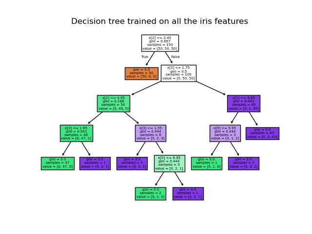
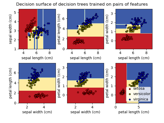
Using the Iris dataset, we can construct a tree as follows:
>>> from sklearn.datasets import load_iris
>>> from sklearn import tree
>>> iris = load_iris()
>>> X, y = iris.data, iris.target
>>> clf = tree.DecisionTreeClassifier()
>>> clf = clf.fit(X, y)
Once trained, you can plot the tree with the plot_tree function:
>>> tree.plot_tree(clf)
[...]
Alternative ways to export trees#
We can also export the tree in Graphviz format using the export_graphviz
exporter. If you use the conda package manager, the graphviz binaries
and the python package can be installed with conda install python-graphviz.
Alternatively binaries for graphviz can be downloaded from the graphviz project homepage,
and the Python wrapper installed from pypi with pip install graphviz.
Below is an example graphviz export of the above tree trained on the entire
iris dataset; the results are saved in an output file iris.pdf:
>>> import graphviz
>>> dot_data = tree.export_graphviz(clf, out_file=None)
>>> graph = graphviz.Source(dot_data)
>>> graph.render("iris")
The export_graphviz exporter also supports a variety of aesthetic
options, including coloring nodes by their class (or value for regression) and
using explicit variable and class names if desired. Jupyter notebooks also
render these plots inline automatically:
>>> dot_data = tree.export_graphviz(clf, out_file=None,
...                      feature_names=iris.feature_names,
...                      class_names=iris.target_names,
...                      filled=True, rounded=True,
...                      special_characters=True)
>>> graph = graphviz.Source(dot_data)
>>> graph

Alternatively, the tree can also be exported in textual format with the
function export_text. This method doesn’t require the installation
of external libraries and is more compact:
>>> from sklearn.datasets import load_iris
>>> from sklearn.tree import DecisionTreeClassifier
>>> from sklearn.tree import export_text
>>> iris = load_iris()
>>> decision_tree = DecisionTreeClassifier(random_state=0, max_depth=2)
>>> decision_tree = decision_tree.fit(iris.data, iris.target)
>>> r = export_text(decision_tree, feature_names=iris['feature_names'])
>>> print(r)
|--- petal width (cm) <= 0.80
|   |--- class: 0
|--- petal width (cm) >  0.80
|   |--- petal width (cm) <= 1.75
|   |   |--- class: 1
|   |--- petal width (cm) >  1.75
|   |   |--- class: 2
Examples
1.10.2. Regression#
Decision trees can also be applied to regression problems, using the
DecisionTreeRegressor class.
As in the classification setting, the fit method will take as argument arrays X and y, only that in this case y is expected to have floating point values instead of integer values:
>>> from sklearn import tree
>>> X = [[0, 0], [2, 2]]
>>> y = [0.5, 2.5]
>>> clf = tree.DecisionTreeRegressor()
>>> clf = clf.fit(X, y)
>>> clf.predict([[1, 1]])
array([0.5])
Examples
1.10.3. Multi-output problems#
A multi-output problem is a supervised learning problem with several outputs
to predict, that is when Y is a 2d array of shape (n_samples, n_outputs).
When there is no correlation between the outputs, a very simple way to solve this kind of problem is to build n independent models, i.e. one for each output, and then to use those models to independently predict each one of the n outputs. However, because it is likely that the output values related to the same input are themselves correlated, an often better way is to build a single model capable of predicting simultaneously all n outputs. First, it requires lower training time since only a single estimator is built. Second, the generalization accuracy of the resulting estimator may often be increased.
With regard to decision trees, this strategy can readily be used to support multi-output problems. This requires the following changes:
Store n output values in leaves, instead of 1;
Use splitting criteria that compute the average reduction across all n outputs.
This module offers support for multi-output problems by implementing this
strategy in both DecisionTreeClassifier and
DecisionTreeRegressor. If a decision tree is fit on an output array Y
of shape (n_samples, n_outputs) then the resulting estimator will:
Output n_output values upon
predict;Output a list of n_output arrays of class probabilities upon
predict_proba.
The use of multi-output trees for regression is demonstrated in Decision Tree Regression. In this example, the input X is a single real value and the outputs Y are the sine and cosine of X.

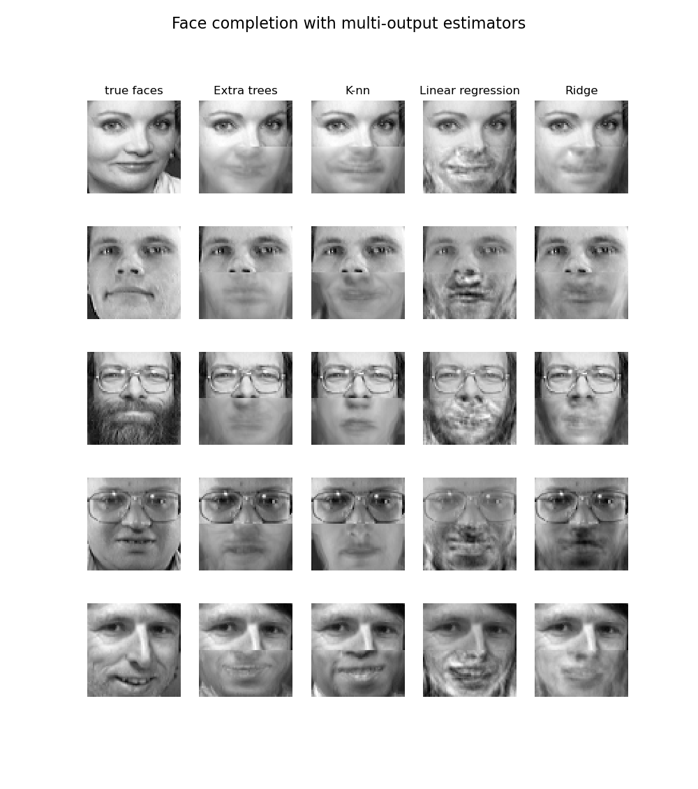
The use of multi-output trees for classification is demonstrated in Face completion with a multi-output estimators. In this example, the inputs X are the pixels of the upper half of faces and the outputs Y are the pixels of the lower half of those faces.
Examples
References
M. Dumont et al, Fast multi-class image annotation with random subwindows and multiple output randomized trees, International Conference on Computer Vision Theory and Applications 2009
1.10.4. Complexity#
The following table shows the worst-case complexity estimates for a balanced binary tree:
Splitter |
Total training cost |
Total inference cost |
|---|---|---|
“best” |
\(\mathcal{O}(n_{features} \, n^2_{samples} \log(n_{samples}))\) |
\(\mathcal{O}(\log(n_{samples}))\) |
“random” |
\(\mathcal{O}(n_{features} \, n^2_{samples})\) |
\(\mathcal{O}(\log(n_{samples}))\) |
In general, the training cost to construct a balanced binary tree at each node is
The first term is the cost of sorting \(n_{samples}\) repeated for \(n_{features}\). The second term is the linear scan over candidate split points to find the feature that offers the largest reduction in the impurity criterion. The latter is sub-leading for the greedy splitter strategy “best”, and is therefore typically discarded.
Regardless of the splitting strategy, after summing the cost over all internal nodes, the total complexity scales linearly with \(n_{nodes}=n_{leaves}-1\), which is \(\mathcal{O}(n_{samples})\) in the worst-case complexity, that is, when the tree is grown until each sample ends up in its own leaf.
Many implementations such as scikit-learn use efficient caching tricks to keep track of the general order of indices at each node such that the features do not need to be re-sorted at each node; hence, the time complexity of these implementations is just \(\mathcal{O}(n_{features}n_{samples}\log(n_{samples}))\) [1].
Inference cost is independent of the splitter strategy. It depends only on the tree depth, \(\mathcal{O}(\text{depth})\). In an approximately balanced binary tree, each split halves the data, and then the number of such halvings grows with the depth as powers of two. If this process continues until each sample is isolated in its own leaf, the resulting depth is \(\mathcal{O}(\log(n_{samples}))\).
References
1.10.5. Tips on practical use#
Decision trees tend to overfit on data with a large number of features. Getting the right ratio of samples to number of features is important, since a tree with few samples in high dimensional space is very likely to overfit.
Consider performing dimensionality reduction (PCA, ICA, or Feature selection) beforehand to give your tree a better chance of finding features that are discriminative.
Understanding the decision tree structure will help in gaining more insights about how the decision tree makes predictions, which is important for understanding the important features in the data.
Visualize your tree as you are training by using the
exportfunction. Usemax_depth=3as an initial tree depth to get a feel for how the tree is fitting to your data, and then increase the depth.Remember that the number of samples required to populate the tree doubles for each additional level the tree grows to. Use
max_depthto control the size of the tree to prevent overfitting.Use
min_samples_splitormin_samples_leafto ensure that multiple samples inform every decision in the tree, by controlling which splits will be considered. A very small number will usually mean the tree will overfit, whereas a large number will prevent the tree from learning the data. Trymin_samples_leaf=5as an initial value. If the sample size varies greatly, a float number can be used as percentage in these two parameters. Whilemin_samples_splitcan create arbitrarily small leaves,min_samples_leafguarantees that each leaf has a minimum size, avoiding low-variance, over-fit leaf nodes in regression problems. For classification with few classes,min_samples_leaf=1is often the best choice.Note that
min_samples_splitconsiders samples directly and independent ofsample_weight, if provided (e.g. a node with m weighted samples is still treated as having exactly m samples). Considermin_weight_fraction_leaformin_impurity_decreaseif accounting for sample weights is required at splits.Balance your dataset before training to prevent the tree from being biased toward the classes that are dominant. Class balancing can be done by sampling an equal number of samples from each class, or preferably by normalizing the sum of the sample weights (
sample_weight) for each class to the same value. Also note that weight-based pre-pruning criteria, such asmin_weight_fraction_leaf, will then be less biased toward dominant classes than criteria that are not aware of the sample weights, likemin_samples_leaf.If the samples are weighted, it will be easier to optimize the tree structure using weight-based pre-pruning criterion such as
min_weight_fraction_leaf, which ensures that leaf nodes contain at least a fraction of the overall sum of the sample weights.All decision trees use
np.float32arrays internally. If training data is not in this format, a copy of the dataset will be made.If the input matrix X is very sparse, it is recommended to convert to sparse
csc_matrixbefore calling fit and sparsecsr_matrixbefore calling predict. Training time can be orders of magnitude faster for a sparse matrix input compared to a dense matrix when features have zero values in most of the samples.
1.10.6. Tree algorithms: ID3, C4.5, C5.0 and CART#
What are all the various decision tree algorithms and how do they differ from each other? Which one is implemented in scikit-learn?
Various decision tree algorithms#
ID3 (Iterative Dichotomiser 3) was developed in 1986 by Ross Quinlan. The algorithm creates a multiway tree, finding for each node (i.e. in a greedy manner) the categorical feature that will yield the largest information gain for categorical targets. Trees are grown to their maximum size and then a pruning step is usually applied to improve the ability of the tree to generalize to unseen data.
C4.5 is the successor to ID3 and removed the restriction that features must be categorical by dynamically defining a discrete attribute (based on numerical variables) that partitions the continuous attribute value into a discrete set of intervals. C4.5 converts the trained trees (i.e. the output of the ID3 algorithm) into sets of if-then rules. The accuracy of each rule is then evaluated to determine the order in which they should be applied. Pruning is done by removing a rule’s precondition if the accuracy of the rule improves without it.
C5.0 is Quinlan’s latest version release under a proprietary license. It uses less memory and builds smaller rulesets than C4.5 while being more accurate.
CART (Classification and Regression Trees) is very similar to C4.5, but it differs in that it supports numerical target variables (regression) and does not compute rule sets. CART constructs binary trees using the feature and threshold that yield the largest information gain at each node.
scikit-learn uses an optimized version of the CART algorithm; however, the scikit-learn implementation does not support categorical variables for now.
1.10.7. Mathematical formulation#
Given training vectors \(x_i \in R^n\), i=1,…, l and a label vector \(y \in R^l\), a decision tree recursively partitions the feature space such that the samples with the same labels or similar target values are grouped together.
Let the data at node \(m\) be represented by \(Q_m\) with \(n_m\) samples. For each candidate split \(\theta = (j, t_m)\) consisting of a feature \(j\) and threshold \(t_m\), partition the data into \(Q_m^{left}(\theta)\) and \(Q_m^{right}(\theta)\) subsets
The quality of a candidate split of node \(m\) is then computed using an impurity function or loss function \(H()\), the choice of which depends on the task being solved (classification or regression)
Select the parameters that minimises the impurity
The strategy to choose the split at each node is controlled by the splitter
parameter:
With the best splitter (default,
splitter='best'), \(\theta^*\) is found by performing a greedy exhaustive search over all available features and all possible thresholds \(t_m\) (i.e. midpoints between sorted, distinct feature values), selecting the pair that exactly minimizes \(G(Q_m, \theta)\).With the random splitter (
splitter='random'), \(\theta^*\) is found by sampling a single random candidate threshold for each available feature. This performs a stochastic approximation of the greedy search, effectively reducing computation time (see Complexity).
After choosing the optimal split \(\theta^*\) at node \(m\), the same splitting procedure is then applied recursively to each partition \(Q_m^{left}(\theta^*)\) and \(Q_m^{right}(\theta^*)\) until a stopping condition is reached, such as:
the maximum allowable depth is reached (
max_depth);\(n_m\) is smaller than
min_samples_split;the impurity decrease for this split is smaller than
min_impurity_decrease.
See the respective estimator docstring for other stopping conditions.
1.10.7.1. Classification criteria#
If a target is a classification outcome taking on values 0,1,…,K-1, for node \(m\), let
be the proportion of class k observations in node \(m\). If \(m\) is a
terminal node, predict_proba for this region is set to \(p_{mk}\).
Common measures of impurity are the following.
Gini:
Log Loss or Entropy:
Shannon entropy#
The entropy criterion computes the Shannon entropy of the possible classes. It takes the class frequencies of the training data points that reached a given leaf \(m\) as their probability. Using the Shannon entropy as tree node splitting criterion is equivalent to minimizing the log loss (also known as cross-entropy and multinomial deviance) between the true labels \(y_i\) and the probabilistic predictions \(T_k(x_i)\) of the tree model \(T\) for class \(k\).
To see this, first recall that the log loss of a tree model \(T\) computed on a dataset \(D\) is defined as follows:
where \(D\) is a training dataset of \(n\) pairs \((x_i, y_i)\).
In a classification tree, the predicted class probabilities within leaf nodes are constant, that is: for all \((x_i, y_i) \in Q_m\), one has: \(T_k(x_i) = p_{mk}\) for each class \(k\).
This property makes it possible to rewrite \(\mathrm{LL}(D, T)\) as the sum of the Shannon entropies computed for each leaf of \(T\) weighted by the number of training data points that reached each leaf:
1.10.7.2. Regression criteria#
If the target is a continuous value, then for node \(m\), common criteria to minimize as for determining locations for future splits are Mean Squared Error (MSE or L2 error), Poisson deviance as well as Mean Absolute Error (MAE or L1 error). MSE and Poisson deviance both set the predicted value of terminal nodes to the learned mean value \(\bar{y}_m\) of the node whereas the MAE sets the predicted value of terminal nodes to the median \(median(y)_m\).
Mean Squared Error:
Mean Poisson deviance:
Setting criterion="poisson" might be a good choice if your target is a count
or a frequency (count per some unit). In any case, \(y >= 0\) is a
necessary condition to use this criterion. For performance reasons the actual
implementation minimizes the half mean poisson deviance, i.e. the mean poisson
deviance divided by 2.
Mean Absolute Error:
Note that it is 3–6× slower to fit than the MSE criterion as of version 1.8.
1.10.8. Missing Values Support#
DecisionTreeClassifier, DecisionTreeRegressor
have built-in support for missing values using splitter='best', where
the splits are determined in a greedy fashion.
ExtraTreeClassifier, and ExtraTreeRegressor have built-in
support for missing values for splitter='random', where the splits
are determined randomly. For more details on how the splitter differs on
non-missing values, see the Forest section.
The criterion supported when there are missing values are
'gini', 'entropy', or 'log_loss', for classification or
'squared_error', 'friedman_mse', or 'poisson' for regression.
First we will describe how DecisionTreeClassifier, DecisionTreeRegressor
handle missing-values in the data.
For each potential threshold on the non-missing data, the splitter will evaluate the split with all the missing values going to the left node or the right node.
Decisions are made as follows:
By default when predicting, the samples with missing values are classified with the class used in the split found during training:
>>> from sklearn.tree import DecisionTreeClassifier
>>> import numpy as np

>>> X = np.array([0, 1, 6, np.nan]).reshape(-1, 1)
>>> y = [0, 0, 1, 1]

>>> tree = DecisionTreeClassifier(random_state=0).fit(X, y)
>>> tree.predict(X)
array([0, 0, 1, 1])
If the criterion evaluation is the same for both nodes, then the tie for missing value at predict time is broken by going to the right node. The splitter also checks the split where all the missing values go to one child and non-missing values go to the other:
>>> from sklearn.tree import DecisionTreeClassifier
>>> import numpy as np

>>> X = np.array([np.nan, -1, np.nan, 1]).reshape(-1, 1)
>>> y = [0, 0, 1, 1]

>>> tree = DecisionTreeClassifier(random_state=0, max_depth=1).fit(X, y)

>>> X_test = np.array([np.nan]).reshape(-1, 1)
>>> tree.predict(X_test)
array([1])
If no missing values are seen during training for a given feature, then during prediction missing values are mapped to the child with the most samples:
>>> from sklearn.tree import DecisionTreeClassifier
>>> import numpy as np

>>> X = np.array([0, 1, 2, 3]).reshape(-1, 1)
>>> y = [0, 1, 1, 1]

>>> tree = DecisionTreeClassifier(random_state=0).fit(X, y)

>>> X_test = np.array([np.nan]).reshape(-1, 1)
>>> tree.predict(X_test)
array([1])
ExtraTreeClassifier, and ExtraTreeRegressor handle missing values
in a slightly different way. When splitting a node, a random threshold will be chosen
to split the non-missing values on. Then the non-missing values will be sent to the
left and right child based on the randomly selected threshold, while the missing
values will also be randomly sent to the left or right child. This is repeated for
every feature considered at each split. The best split among these is chosen.
During prediction, the treatment of missing-values is the same as that of the decision tree:
By default when predicting, the samples with missing values are classified with the class used in the split found during training.
If no missing values are seen during training for a given feature, then during prediction missing values are mapped to the child with the most samples.
1.10.9. Minimal Cost-Complexity Pruning#
Minimal cost-complexity pruning is an algorithm used to prune a tree to avoid over-fitting, described in Chapter 3 of [BRE]. This algorithm is parameterized by \(\alpha\ge0\) known as the complexity parameter. The complexity parameter is used to define the cost-complexity measure, \(R_\alpha(T)\) of a given tree \(T\):
where \(|\widetilde{T}|\) is the number of terminal nodes in \(T\) and \(R(T)\) is traditionally defined as the total misclassification rate of the terminal nodes. Alternatively, scikit-learn uses the total sample weighted impurity of the terminal nodes for \(R(T)\). As shown above, the impurity of a node depends on the criterion. Minimal cost-complexity pruning finds the subtree of \(T\) that minimizes \(R_\alpha(T)\).
The cost complexity measure of a single node is
\(R_\alpha(t)=R(t)+\alpha\). The branch, \(T_t\), is defined to be a
tree where node \(t\) is its root. In general, the impurity of a node
is greater than the sum of impurities of its terminal nodes,
\(R(T_t)<R(t)\). However, the cost complexity measure of a node,
\(t\), and its branch, \(T_t\), can be equal depending on
\(\alpha\). We define the effective \(\alpha\) of a node to be the
value where they are equal, \(R_\alpha(T_t)=R_\alpha(t)\) or
\(\alpha_{eff}(t)=\frac{R(t)-R(T_t)}{|T|-1}\). A non-terminal node
with the smallest value of \(\alpha_{eff}\) is the weakest link and will
be pruned. This process stops when the pruned tree’s minimal
\(\alpha_{eff}\) is greater than the ccp_alpha parameter.
Examples
References
L. Breiman, J. Friedman, R. Olshen, and C. Stone. Classification and Regression Trees. Wadsworth, Belmont, CA, 1984.
J.R. Quinlan. C4. 5: programs for machine learning. Morgan Kaufmann, 1993.
T. Hastie, R. Tibshirani and J. Friedman. Elements of Statistical Learning, Springer, 2009.