3.1. Cross-validation: evaluating estimator performance#
Learning the parameters of a prediction function and testing it on the
same data is a methodological mistake: a model that would just repeat
the labels of the samples that it has just seen would have a perfect
score but would fail to predict anything useful on yet-unseen data.
This situation is called overfitting.
To avoid it, it is common practice when performing
a (supervised) machine learning experiment
to hold out part of the available data as a test set X_test, y_test.
Note that the word “experiment” is not intended
to denote academic use only,
because even in commercial settings
machine learning usually starts out experimentally.
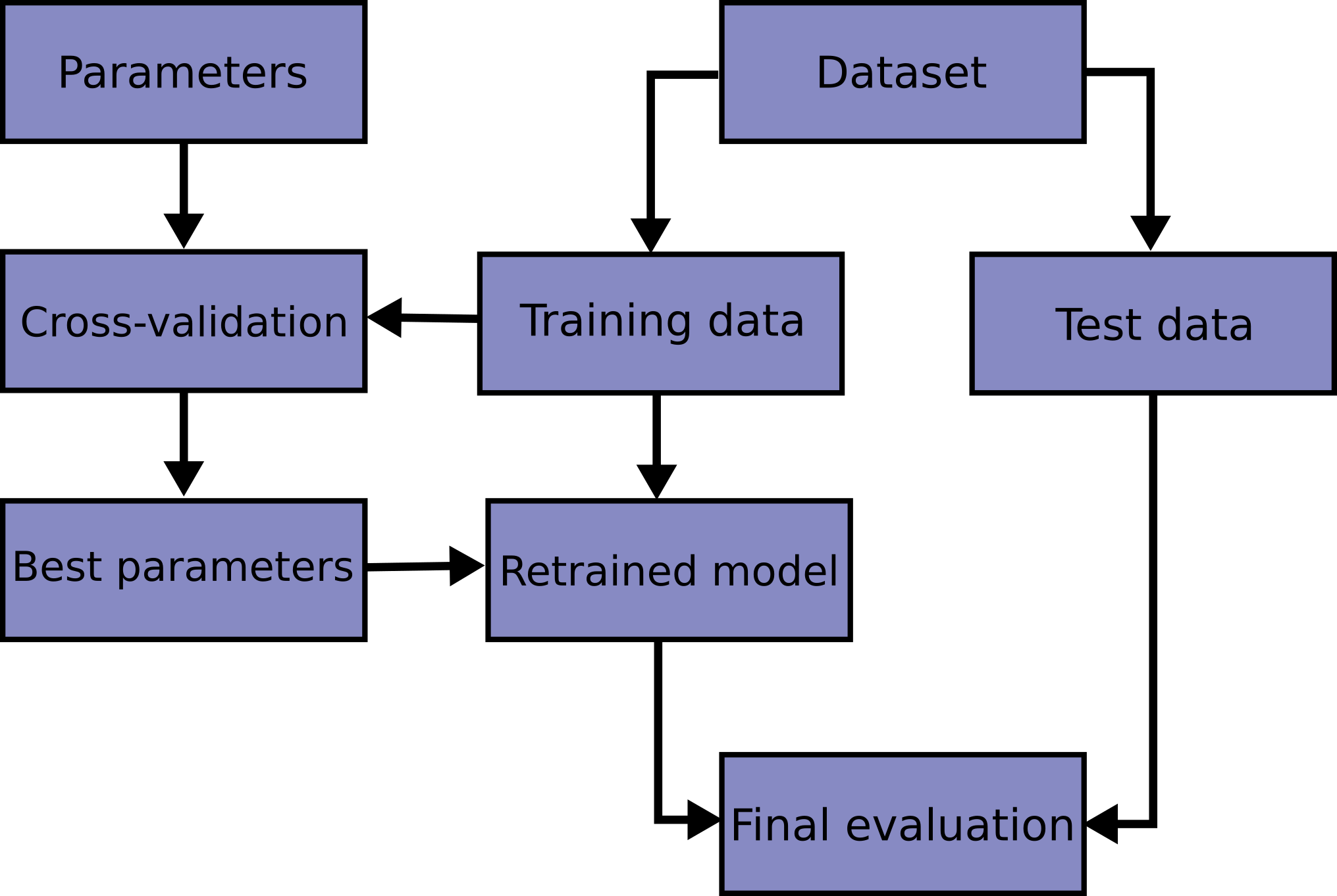
Here is a flowchart of typical cross validation workflow in model training.
The best parameters can be determined by
grid search techniques.
In scikit-learn a random split into training and test sets
can be quickly computed with the train_test_split helper function.
Let’s load the iris data set to fit a linear support vector machine on it:
>>> import numpy as np
>>> from sklearn.model_selection import train_test_split
>>> from sklearn import datasets
>>> from sklearn import svm

>>> X, y = datasets.load_iris(return_X_y=True)
>>> X.shape, y.shape
((150, 4), (150,))
We can now quickly sample a training set while holding out 40% of the data for testing (evaluating) our classifier:
>>> X_train, X_test, y_train, y_test = train_test_split(
...     X, y, test_size=0.4, random_state=0)

>>> X_train.shape, y_train.shape
((90, 4), (90,))
>>> X_test.shape, y_test.shape
((60, 4), (60,))

>>> clf = svm.SVC(kernel='linear', C=1).fit(X_train, y_train)
>>> clf.score(X_test, y_test)
0.96
When evaluating different settings (“hyperparameters”) for estimators,
such as the C setting that must be manually set for an SVM,
there is still a risk of overfitting on the test set
because the parameters can be tweaked until the estimator performs optimally.
This way, knowledge about the test set can “leak” into the model
and evaluation metrics no longer report on generalization performance.
To solve this problem, yet another part of the dataset can be held out
as a so-called “validation set”: training proceeds on the training set,
after which evaluation is done on the validation set,
and when the experiment seems to be successful,
final evaluation can be done on the test set.
However, by partitioning the available data into three sets, we drastically reduce the number of samples which can be used for learning the model, and the results can depend on a particular random choice for the pair of (train, validation) sets.
A solution to this problem is a procedure called cross-validation (CV for short). A test set should still be held out for final evaluation, but the validation set is no longer needed when doing CV. In the basic approach, called k-fold CV, the training set is split into k smaller sets (other approaches are described below, but generally follow the same principles). The following procedure is followed for each of the k “folds”:
A model is trained using \(k-1\) of the folds as training data;
the resulting model is validated on the remaining part of the data (i.e., it is used as a test set to compute a performance measure such as accuracy).
The performance measure reported by k-fold cross-validation is then the average of the values computed in the loop. This approach can be computationally expensive, but does not waste too much data (as is the case when fixing an arbitrary validation set), which is a major advantage in problems such as inverse inference where the number of samples is very small.

3.1.1. Computing cross-validated metrics#
The simplest way to use cross-validation is to call the
cross_val_score helper function on the estimator and the dataset.
The following example demonstrates how to estimate the accuracy of a linear kernel support vector machine on the iris dataset by splitting the data, fitting a model and computing the score 5 consecutive times (with different splits each time):
>>> from sklearn.model_selection import cross_val_score
>>> clf = svm.SVC(kernel='linear', C=1, random_state=42)
>>> scores = cross_val_score(clf, X, y, cv=5)
>>> scores
array([0.96, 1. , 0.96, 0.96, 1. ])
The mean score and the standard deviation are hence given by:
>>> print("%0.2f accuracy with a standard deviation of %0.2f" % (scores.mean(), scores.std()))
0.98 accuracy with a standard deviation of 0.02
By default, the score computed at each CV iteration is the score
method of the estimator. It is possible to change this by using the
scoring parameter:
>>> from sklearn import metrics
>>> scores = cross_val_score(
...     clf, X, y, cv=5, scoring='f1_macro')
>>> scores
array([0.96, 1., 0.96, 0.96, 1.])
See The scoring parameter: defining model evaluation rules for details. In the case of the Iris dataset, the samples are balanced across target classes hence the accuracy and the F1-score are almost equal.
When the cv argument is an integer, cross_val_score uses the
KFold or StratifiedKFold strategies by default, the latter
being used if the estimator derives from ClassifierMixin.
It is also possible to use other cross validation strategies by passing a cross validation iterator instead, for instance:
>>> from sklearn.model_selection import ShuffleSplit
>>> n_samples = X.shape[0]
>>> cv = ShuffleSplit(n_splits=5, test_size=0.3, random_state=0)
>>> cross_val_score(clf, X, y, cv=cv)
array([0.977, 0.977, 1., 0.955, 1.])
Another option is to use an iterable yielding (train, test) splits as arrays of indices, for example:
>>> def custom_cv_2folds(X):
...     n = X.shape[0]
...     i = 1
...     while i <= 2:
...         idx = np.arange(n * (i - 1) / 2, n * i / 2, dtype=int)
...         yield idx, idx
...         i += 1
...
>>> custom_cv = custom_cv_2folds(X)
>>> cross_val_score(clf, X, y, cv=custom_cv)
array([1.        , 0.973])
Data transformation with held-out data#
Just as it is important to test a predictor on data held-out from training, preprocessing (such as standardization, feature selection, etc.) and similar data transformations similarly should be learnt from a training set and applied to held-out data for prediction:
>>> from sklearn import preprocessing
>>> X_train, X_test, y_train, y_test = train_test_split(
...     X, y, test_size=0.4, random_state=0)
>>> scaler = preprocessing.StandardScaler().fit(X_train)
>>> X_train_transformed = scaler.transform(X_train)
>>> clf = svm.SVC(C=1).fit(X_train_transformed, y_train)
>>> X_test_transformed = scaler.transform(X_test)
>>> clf.score(X_test_transformed, y_test)
0.9333
A Pipeline makes it easier to compose
estimators, providing this behavior under cross-validation:
>>> from sklearn.pipeline import make_pipeline
>>> clf = make_pipeline(preprocessing.StandardScaler(), svm.SVC(C=1))
>>> cross_val_score(clf, X, y, cv=cv)
array([0.977, 0.933, 0.955, 0.933, 0.977])
3.1.1.1. The cross_validate function and multiple metric evaluation#
The cross_validate function differs from cross_val_score in
two ways:
It allows specifying multiple metrics for evaluation.
It returns a dict containing fit-times, score-times (and optionally training scores, fitted estimators, train-test split indices) in addition to the test score.
For single metric evaluation, where the scoring parameter is a string,
callable or None, the keys will be - ['test_score', 'fit_time', 'score_time']
And for multiple metric evaluation, the return value is a dict with the
following keys -
['test_<scorer1_name>', 'test_<scorer2_name>', 'test_<scorer...>', 'fit_time', 'score_time']
return_train_score is set to False by default to save computation time.
To evaluate the scores on the training set as well you need to set it to
True. You may also retain the estimator fitted on each training set by
setting return_estimator=True. Similarly, you may set
return_indices=True to retain the training and testing indices used to split
the dataset into train and test sets for each cv split.
The multiple metrics can be specified either as a list, tuple or set of predefined scorer names:
>>> from sklearn.model_selection import cross_validate
>>> from sklearn.metrics import recall_score
>>> scoring = ['precision_macro', 'recall_macro']
>>> clf = svm.SVC(kernel='linear', C=1, random_state=0)
>>> scores = cross_validate(clf, X, y, scoring=scoring)
>>> sorted(scores.keys())
['fit_time', 'score_time', 'test_precision_macro', 'test_recall_macro']
>>> scores['test_recall_macro']
array([0.96, 1., 0.96, 0.96, 1.])
Or as a dict mapping scorer name to a predefined or custom scoring function:
>>> from sklearn.metrics import make_scorer
>>> scoring = {'prec_macro': 'precision_macro',
...            'rec_macro': make_scorer(recall_score, average='macro')}
>>> scores = cross_validate(clf, X, y, scoring=scoring,
...                         cv=5, return_train_score=True)
>>> sorted(scores.keys())
['fit_time', 'score_time', 'test_prec_macro', 'test_rec_macro',
 'train_prec_macro', 'train_rec_macro']
>>> scores['train_rec_macro']
array([0.97, 0.97, 0.99, 0.98, 0.98])
Here is an example of cross_validate using a single metric:
>>> scores = cross_validate(clf, X, y,
...                         scoring='precision_macro', cv=5,
...                         return_estimator=True)
>>> sorted(scores.keys())
['estimator', 'fit_time', 'score_time', 'test_score']
3.1.1.2. Obtaining predictions by cross-validation#
The function cross_val_predict has a similar interface to
cross_val_score, but returns, for each element in the input, the
prediction that was obtained for that element when it was in the test set. Only
cross-validation strategies that assign all elements to a test set exactly once
can be used (otherwise, an exception is raised).
Warning
Note on inappropriate usage of cross_val_predict
The result of cross_val_predict may be different from those
obtained using cross_val_score as the elements are grouped in
different ways. The function cross_val_score takes an average
over cross-validation folds, whereas cross_val_predict simply
returns the labels (or probabilities) from several distinct models
undistinguished. Thus, cross_val_predict is not an appropriate
measure of generalization error.
- The function
cross_val_predictis appropriate for: Visualization of predictions obtained from different models.
Model blending: When predictions of one supervised estimator are used to train another estimator in ensemble methods.
The available cross validation iterators are introduced in the following section.
Examples
3.1.2. Cross validation iterators#
The following sections list utilities to generate indices that can be used to generate dataset splits according to different cross validation strategies.
3.1.2.1. Cross-validation iterators for i.i.d. data#
Assuming that some data is Independent and Identically Distributed (i.i.d.) is making the assumption that all samples stem from the same generative process and that the generative process is assumed to have no memory of past generated samples.
The following cross-validators can be used in such cases.
Note
While i.i.d. data is a common assumption in machine learning theory, it rarely holds in practice. If one knows that the samples have been generated using a time-dependent process, it is safer to use a time-series aware cross-validation scheme. Similarly, if we know that the generative process has a group structure (samples collected from different subjects, experiments, measurement devices), it is safer to use group-wise cross-validation.
3.1.2.1.1. K-fold#
KFold divides all the samples in \(k\) groups of samples,
called folds (if \(k = n\), this is equivalent to the Leave One
Out strategy), of equal sizes (if possible). The prediction function is
learned using \(k - 1\) folds, and the fold left out is used for test.
Example of 2-fold cross-validation on a dataset with 4 samples:
>>> import numpy as np
>>> from sklearn.model_selection import KFold

>>> X = ["a", "b", "c", "d"]
>>> kf = KFold(n_splits=2)
>>> for train, test in kf.split(X):
...     print("%s %s" % (train, test))
[2 3] [0 1]
[0 1] [2 3]
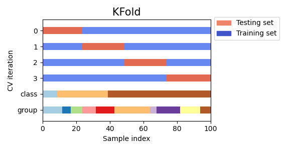
Here is a visualization of the cross-validation behavior. Note that
KFold is not affected by classes or groups.
Each fold is constituted by two arrays: the first one is related to the training set, and the second one to the test set. Thus, one can create the training/test sets using numpy indexing:
>>> X = np.array([[0., 0.], [1., 1.], [-1., -1.], [2., 2.]])
>>> y = np.array([0, 1, 0, 1])
>>> X_train, X_test, y_train, y_test = X[train], X[test], y[train], y[test]
3.1.2.1.2. Repeated K-Fold#
RepeatedKFold repeats KFold \(n\) times, producing different splits in
each repetition.
Example of 2-fold K-Fold repeated 2 times:
>>> import numpy as np
>>> from sklearn.model_selection import RepeatedKFold
>>> X = np.array([[1, 2], [3, 4], [1, 2], [3, 4]])
>>> random_state = 12883823
>>> rkf = RepeatedKFold(n_splits=2, n_repeats=2, random_state=random_state)
>>> for train, test in rkf.split(X):
...     print("%s %s" % (train, test))
...
[2 3] [0 1]
[0 1] [2 3]
[0 2] [1 3]
[1 3] [0 2]
Similarly, RepeatedStratifiedKFold repeats StratifiedKFold \(n\) times
with different randomization in each repetition.
3.1.2.1.3. Leave One Out (LOO)#
LeaveOneOut (or LOO) is a simple cross-validation. Each learning
set is created by taking all the samples except one, the test set being
the sample left out. Thus, for \(n\) samples, we have \(n\) different
training sets and \(n\) different test sets. This cross-validation
procedure does not waste much data as only one sample is removed from the
training set:
>>> from sklearn.model_selection import LeaveOneOut

>>> X = [1, 2, 3, 4]
>>> loo = LeaveOneOut()
>>> for train, test in loo.split(X):
...     print("%s %s" % (train, test))
[1 2 3] [0]
[0 2 3] [1]
[0 1 3] [2]
[0 1 2] [3]
Potential users of LOO for model selection should weigh a few known caveats. When compared with \(k\)-fold cross validation, one builds \(n\) models from \(n\) samples instead of \(k\) models, where \(n > k\). Moreover, each is trained on \(n - 1\) samples rather than \((k-1) n / k\). In both ways, assuming \(k\) is not too large and \(k < n\), LOO is more computationally expensive than \(k\)-fold cross validation.
In terms of accuracy, LOO often results in high variance as an estimator for the test error. Intuitively, since \(n - 1\) of the \(n\) samples are used to build each model, models constructed from folds are virtually identical to each other and to the model built from the entire training set.
However, if the learning curve is steep for the training size in question, then 5 or 10-fold cross validation can overestimate the generalization error.
As a general rule, most authors and empirical evidence suggest that 5 or 10-fold cross validation should be preferred to LOO.
References#
http://www.faqs.org/faqs/ai-faq/neural-nets/part3/section-12.html;
T. Hastie, R. Tibshirani, J. Friedman, The Elements of Statistical Learning, Springer 2009
L. Breiman, P. Spector Submodel selection and evaluation in regression: The X-random case, International Statistical Review 1992;
R. Kohavi, A Study of Cross-Validation and Bootstrap for Accuracy Estimation and Model Selection, Intl. Jnt. Conf. AI
R. Bharat Rao, G. Fung, R. Rosales, On the Dangers of Cross-Validation. An Experimental Evaluation, SIAM 2008;
G. James, D. Witten, T. Hastie, R. Tibshirani, An Introduction to Statistical Learning, Springer 2013.
3.1.2.1.4. Leave P Out (LPO)#
LeavePOut is very similar to LeaveOneOut as it creates all
the possible training/test sets by removing \(p\) samples from the complete
set. For \(n\) samples, this produces \({n \choose p}\) train-test
pairs. Unlike LeaveOneOut and KFold, the test sets will
overlap for \(p > 1\).
Example of Leave-2-Out on a dataset with 4 samples:
>>> from sklearn.model_selection import LeavePOut

>>> X = np.ones(4)
>>> lpo = LeavePOut(p=2)
>>> for train, test in lpo.split(X):
...     print("%s %s" % (train, test))
[2 3] [0 1]
[1 3] [0 2]
[1 2] [0 3]
[0 3] [1 2]
[0 2] [1 3]
[0 1] [2 3]
3.1.2.1.5. Random permutations cross-validation a.k.a. Shuffle & Split#
The ShuffleSplit iterator will generate a user defined number of
independent train / test dataset splits. Samples are first shuffled and
then split into a pair of train and test sets.
It is possible to control the randomness for reproducibility of the
results by explicitly seeding the random_state pseudo random number
generator.
Here is a usage example:
>>> from sklearn.model_selection import ShuffleSplit
>>> X = np.arange(10)
>>> ss = ShuffleSplit(n_splits=5, test_size=0.25, random_state=0)
>>> for train_index, test_index in ss.split(X):
...     print("%s %s" % (train_index, test_index))
[9 1 6 7 3 0 5] [2 8 4]
[2 9 8 0 6 7 4] [3 5 1]
[4 5 1 0 6 9 7] [2 3 8]
[2 7 5 8 0 3 4] [6 1 9]
[4 1 0 6 8 9 3] [5 2 7]
Here is a visualization of the cross-validation behavior. Note that
ShuffleSplit is not affected by classes or groups.
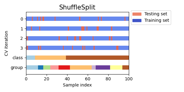
ShuffleSplit is thus a good alternative to KFold cross
validation that allows a finer control on the number of iterations and
the proportion of samples on each side of the train / test split.
3.1.2.2. Cross-validation iterators with stratification based on class labels#
Some classification tasks can naturally exhibit rare classes: for instance,
there could be orders of magnitude more negative observations than positive
observations (e.g. medical screening, fraud detection, etc). As a result,
cross-validation splitting can generate train or validation folds without any
occurrence of a particular class. This typically leads to undefined
classification metrics (e.g. ROC AUC), exceptions raised when attempting to
call fit or missing columns in the output of the predict_proba or
decision_function methods of multiclass classifiers trained on different
folds.
To mitigate such problems, splitters such as StratifiedKFold and
StratifiedShuffleSplit implement stratified sampling to ensure that
relative class frequencies are approximately preserved in each fold.
Note
Stratified sampling was introduced in scikit-learn to workaround the aforementioned engineering problems rather than solve a statistical one.
Stratification makes cross-validation folds more homogeneous, and as a result hides some of the variability inherent to fitting models with a limited number of observations.
As a result, stratification can artificially shrink the spread of the metric measured across cross-validation iterations: the inter-fold variability does no longer reflect the uncertainty in the performance of classifiers in the presence of rare classes.
3.1.2.2.1. Stratified K-fold#
StratifiedKFold is a variation of K-fold which returns stratified
folds: each set contains approximately the same percentage of samples of each
target class as the complete set.
Here is an example of stratified 3-fold cross-validation on a dataset with 50 samples from
two unbalanced classes. We show the number of samples in each class and compare with
KFold.
>>> from sklearn.model_selection import StratifiedKFold, KFold
>>> import numpy as np
>>> X, y = np.ones((50, 1)), np.hstack(([0] * 45, [1] * 5))
>>> skf = StratifiedKFold(n_splits=3)
>>> for train, test in skf.split(X, y):
...     print('train -  {}   |   test -  {}'.format(
...         np.bincount(y[train]), np.bincount(y[test])))
train -  [30  3]   |   test -  [15  2]
train -  [30  3]   |   test -  [15  2]
train -  [30  4]   |   test -  [15  1]
>>> kf = KFold(n_splits=3)
>>> for train, test in kf.split(X, y):
...     print('train -  {}   |   test -  {}'.format(
...         np.bincount(y[train]), np.bincount(y[test])))
train -  [28  5]   |   test -  [17]
train -  [28  5]   |   test -  [17]
train -  [34]   |   test -  [11  5]
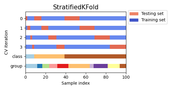
We can see that StratifiedKFold preserves the class ratios
(approximately 1 / 10) in both train and test datasets.
Here is a visualization of the cross-validation behavior.
RepeatedStratifiedKFold can be used to repeat Stratified K-Fold n times
with different randomization in each repetition.
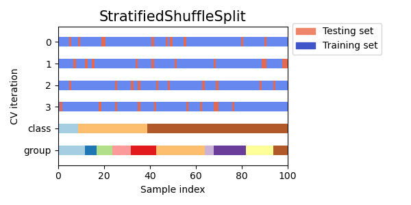
3.1.2.2.2. Stratified Shuffle Split#
StratifiedShuffleSplit is a variation of ShuffleSplit, which returns
stratified splits, i.e. which creates splits by preserving the same
percentage for each target class as in the complete set.
Here is a visualization of the cross-validation behavior.
3.1.2.3. Predefined fold-splits / Validation-sets#
For some datasets, a pre-defined split of the data into training- and
validation fold or into several cross-validation folds already
exists. Using PredefinedSplit it is possible to use these folds
e.g. when searching for hyperparameters.
For example, when using a validation set, set the test_fold to 0 for all
samples that are part of the validation set, and to -1 for all other samples.
3.1.2.4. Cross-validation iterators for grouped data#
The i.i.d. assumption is broken if the underlying generative process yields groups of dependent samples.
Such a grouping of data is domain specific. An example would be when there is medical data collected from multiple patients, with multiple samples taken from each patient. And such data is likely to be dependent on the individual group. In our example, the patient id for each sample will be its group identifier.
In this case we would like to know if a model trained on a particular set of groups generalizes well to the unseen groups. To measure this, we need to ensure that all the samples in the validation fold come from groups that are not represented at all in the paired training fold.
The following cross-validation splitters can be used to do that.
The grouping identifier for the samples is specified via the groups
parameter.
3.1.2.4.1. Group K-fold#
GroupKFold is a variation of K-fold which ensures that the same group is
not represented in both testing and training sets. For example if the data is
obtained from different subjects with several samples per-subject and if the
model is flexible enough to learn from highly person specific features it
could fail to generalize to new subjects. GroupKFold makes it possible
to detect this kind of overfitting situations.
Imagine you have three subjects, each with an associated number from 1 to 3:
>>> from sklearn.model_selection import GroupKFold

>>> X = [0.1, 0.2, 2.2, 2.4, 2.3, 4.55, 5.8, 8.8, 9, 10]
>>> y = ["a", "b", "b", "b", "c", "c", "c", "d", "d", "d"]
>>> groups = [1, 1, 1, 2, 2, 2, 3, 3, 3, 3]

>>> gkf = GroupKFold(n_splits=3)
>>> for train, test in gkf.split(X, y, groups=groups):
...     print("%s %s" % (train, test))
[0 1 2 3 4 5] [6 7 8 9]
[0 1 2 6 7 8 9] [3 4 5]
[3 4 5 6 7 8 9] [0 1 2]
Each subject is in a different testing fold, and the same subject is never in
both testing and training. Notice that the folds do not have exactly the same
size due to the imbalance in the data. If class proportions must be balanced
across folds, StratifiedGroupKFold is a better option.
Here is a visualization of the cross-validation behavior.
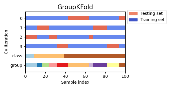
Similar to KFold, the test sets from GroupKFold will form a
complete partition of all the data.
While GroupKFold attempts to place the same number of samples in each
fold when shuffle=False, when shuffle=True it attempts to place an equal
number of distinct groups in each fold (but does not account for group sizes).
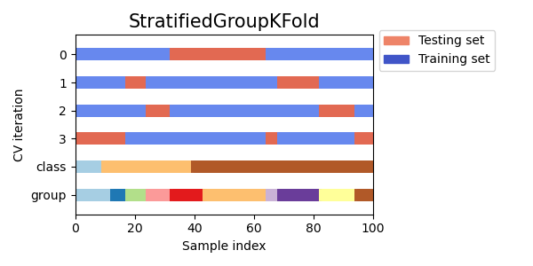
3.1.2.4.2. StratifiedGroupKFold#
StratifiedGroupKFold is a cross-validation scheme that combines both
StratifiedKFold and GroupKFold. The idea is to try to
preserve the distribution of classes in each split while keeping each group
within a single split. That might be useful when you have an unbalanced
dataset so that using just GroupKFold might produce skewed splits.
Example:
>>> from sklearn.model_selection import StratifiedGroupKFold
>>> X = list(range(18))
>>> y = [1] * 6 + [0] * 12
>>> groups = [1, 2, 3, 3, 4, 4, 1, 1, 2, 2, 3, 4, 5, 5, 5, 6, 6, 6]
>>> sgkf = StratifiedGroupKFold(n_splits=3)
>>> for train, test in sgkf.split(X, y, groups=groups):
...     print("%s %s" % (train, test))
[ 0  2  3  4  5  6  7 10 11 15 16 17] [ 1  8  9 12 13 14]
[ 0  1  4  5  6  7  8  9 11 12 13 14] [ 2  3 10 15 16 17]
[ 1  2  3  8  9 10 12 13 14 15 16 17] [ 0  4  5  6  7 11]
Implementation notes#
With the current implementation full shuffle is not possible in most scenarios. When shuffle=True, the following happens:
All groups are shuffled.
Groups are sorted by standard deviation of classes using stable sort.
Sorted groups are iterated over and assigned to folds.
That means that only groups with the same standard deviation of class distribution will be shuffled, which might be useful when each group has only a single class.
The algorithm greedily assigns each group to one of n_splits test sets, choosing the test set that minimises the variance in class distribution across test sets. Group assignment proceeds from groups with highest to lowest variance in class frequency, i.e. large groups peaked on one or few classes are assigned first.
This split is suboptimal in a sense that it might produce imbalanced splits even if perfect stratification is possible. If you have relatively close distribution of classes in each group, using
GroupKFoldis better.
Here is a visualization of cross-validation behavior for uneven groups:
3.1.2.4.3. Leave One Group Out#
LeaveOneGroupOut is a cross-validation scheme where each split holds
out samples belonging to one specific group. Group information is
provided via an array that encodes the group of each sample.
Each training set is thus constituted by all the samples except the ones
related to a specific group. This is the same as LeavePGroupsOut with
n_groups=1 and the same as GroupKFold with n_splits equal to the
number of unique labels passed to the groups parameter.
For example, in the cases of multiple experiments, LeaveOneGroupOut
can be used to create a cross-validation based on the different experiments:
we create a training set using the samples of all the experiments except one:
>>> from sklearn.model_selection import LeaveOneGroupOut

>>> X = [1, 5, 10, 50, 60, 70, 80]
>>> y = [0, 1, 1, 2, 2, 2, 2]
>>> groups = [1, 1, 2, 2, 3, 3, 3]
>>> logo = LeaveOneGroupOut()
>>> for train, test in logo.split(X, y, groups=groups):
...     print("%s %s" % (train, test))
[2 3 4 5 6] [0 1]
[0 1 4 5 6] [2 3]
[0 1 2 3] [4 5 6]
Another common application is to use time information: for instance the groups could be the year of collection of the samples and thus allow for cross-validation against time-based splits.
3.1.2.4.4. Leave P Groups Out#
LeavePGroupsOut is similar to LeaveOneGroupOut, but removes
samples related to \(P\) groups for each training/test set. All possible
combinations of \(P\) groups are left out, meaning test sets will overlap
for \(P>1\).
Example of Leave-2-Group Out:
>>> from sklearn.model_selection import LeavePGroupsOut

>>> X = np.arange(6)
>>> y = [1, 1, 1, 2, 2, 2]
>>> groups = [1, 1, 2, 2, 3, 3]
>>> lpgo = LeavePGroupsOut(n_groups=2)
>>> for train, test in lpgo.split(X, y, groups=groups):
...     print("%s %s" % (train, test))
[4 5] [0 1 2 3]
[2 3] [0 1 4 5]
[0 1] [2 3 4 5]
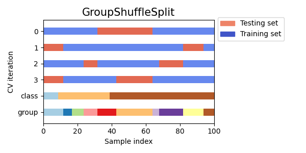
3.1.2.4.5. Group Shuffle Split#
The GroupShuffleSplit iterator behaves as a combination of
ShuffleSplit and LeavePGroupsOut, and generates a
sequence of randomized partitions in which a subset of groups are held
out for each split. Each train/test split is performed independently meaning
there is no guaranteed relationship between successive test sets.
Here is a usage example:
>>> from sklearn.model_selection import GroupShuffleSplit

>>> X = [0.1, 0.2, 2.2, 2.4, 2.3, 4.55, 5.8, 0.001]
>>> y = ["a", "b", "b", "b", "c", "c", "c", "a"]
>>> groups = [1, 1, 2, 2, 3, 3, 4, 4]
>>> gss = GroupShuffleSplit(n_splits=4, test_size=0.5, random_state=0)
>>> for train, test in gss.split(X, y, groups=groups):
...     print("%s %s" % (train, test))
...
[0 1 2 3] [4 5 6 7]
[2 3 6 7] [0 1 4 5]
[2 3 4 5] [0 1 6 7]
[4 5 6 7] [0 1 2 3]
Here is a visualization of the cross-validation behavior.
This class is useful when the behavior of LeavePGroupsOut is
desired, but the number of groups is large enough that generating all
possible partitions with \(P\) groups withheld would be prohibitively
expensive. In such a scenario, GroupShuffleSplit provides
a random sample (with replacement) of the train / test splits
generated by LeavePGroupsOut.
3.1.2.5. Using cross-validation iterators to split train and test#
The above group cross-validation functions may also be useful for splitting a
dataset into training and testing subsets. Note that the convenience
function train_test_split is a wrapper around ShuffleSplit
and thus only allows for stratified splitting (using the class labels)
and cannot account for groups.
To perform the train and test split, use the indices for the train and test
subsets yielded by the generator output by the split() method of the
cross-validation splitter. For example:
>>> import numpy as np
>>> from sklearn.model_selection import GroupShuffleSplit

>>> X = np.array([0.1, 0.2, 2.2, 2.4, 2.3, 4.55, 5.8, 0.001])
>>> y = np.array(["a", "b", "b", "b", "c", "c", "c", "a"])
>>> groups = np.array([1, 1, 2, 2, 3, 3, 4, 4])
>>> train_indx, test_indx = next(
...     GroupShuffleSplit(random_state=7).split(X, y, groups)
... )
>>> X_train, X_test, y_train, y_test = \
...     X[train_indx], X[test_indx], y[train_indx], y[test_indx]
>>> X_train.shape, X_test.shape
((6,), (2,))
>>> np.unique(groups[train_indx]), np.unique(groups[test_indx])
(array([1, 2, 4]), array([3]))
3.1.2.6. Cross validation of time series data#
Time series data is characterized by the correlation between observations
that are near in time (autocorrelation). However, classical
cross-validation techniques such as KFold and
ShuffleSplit assume the samples are independent and
identically distributed, and would result in unreasonable correlation
between training and testing instances (yielding poor estimates of
generalization error) on time series data. Therefore, it is very important
to evaluate our model for time series data on the “future” observations
least like those that are used to train the model. To achieve this, one
solution is provided by TimeSeriesSplit.
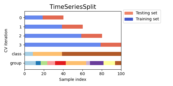
3.1.2.6.1. Time Series Split#
TimeSeriesSplit is a variation of k-fold which
returns first \(k\) folds as train set and the \((k+1)\) th
fold as test set. Note that unlike standard cross-validation methods,
successive training sets are supersets of those that come before them.
Also, it adds all surplus data to the first training partition, which
is always used to train the model.
This class can be used to cross-validate time series data samples that are observed at fixed time intervals. Indeed, the folds must represent the same duration, in order to have comparable metrics across folds.
Example of 3-split time series cross-validation on a dataset with 6 samples:
>>> from sklearn.model_selection import TimeSeriesSplit

>>> X = np.array([[1, 2], [3, 4], [1, 2], [3, 4], [1, 2], [3, 4]])
>>> y = np.array([1, 2, 3, 4, 5, 6])
>>> tscv = TimeSeriesSplit(n_splits=3)
>>> print(tscv)
TimeSeriesSplit(gap=0, max_train_size=None, n_splits=3, test_size=None)
>>> for train, test in tscv.split(X):
...     print("%s %s" % (train, test))
[0 1 2] [3]
[0 1 2 3] [4]
[0 1 2 3 4] [5]
Here is a visualization of the cross-validation behavior.
3.1.3. A note on shuffling#
If the data ordering is not arbitrary (e.g. samples with the same class label are contiguous), shuffling it first may be essential to get a meaningful cross-validation result. However, the opposite may be true if the samples are not independently and identically distributed. For example, if samples correspond to news articles, and are ordered by their time of publication, then shuffling the data will likely lead to a model that is overfit and an inflated validation score: it will be tested on samples that are artificially similar (close in time) to training samples.
Some cross validation iterators, such as KFold, have an inbuilt option
to shuffle the data indices before splitting them. Note that:
This consumes less memory than shuffling the data directly.
By default no shuffling occurs, including for the (stratified) K fold cross-validation performed by specifying
cv=some_integertocross_val_score, grid search, etc. Keep in mind thattrain_test_splitstill returns a random split.The
random_stateparameter defaults toNone, meaning that the shuffling will be different every timeKFold(..., shuffle=True)is iterated. However,GridSearchCVwill use the same shuffling for each set of parameters validated by a single call to itsfitmethod.To get identical results for each split, set
random_stateto an integer.
For more details on how to control the randomness of cv splitters and avoid common pitfalls, see Controlling randomness.
3.1.4. Cross validation and model selection#
Cross validation iterators can also be used to directly perform model selection using Grid Search for the optimal hyperparameters of the model. This is the topic of the next section: Tuning the hyper-parameters of an estimator.
3.1.5. Permutation test score#
permutation_test_score offers another way
to evaluate the performance of a predictor. It provides a
permutation-based p-value, which represents how likely an observed performance of the
estimator would be obtained by chance. The null hypothesis in this test is
that the estimator fails to leverage any statistical dependency between the
features and the targets to make correct predictions on left-out data.
permutation_test_score generates a null
distribution by calculating n_permutations different permutations of the
data. In each permutation the target values are randomly shuffled, thereby removing
any dependency between the features and the targets. The p-value output is the fraction
of permutations whose cross-validation score is better or equal than the true score
without permuting targets. For reliable results n_permutations should typically be
larger than 100 and cv between 3-10 folds.
A low p-value provides evidence that the dataset contains some real dependency between features and targets and that the estimator was able to utilize this dependency to obtain good results. A high p-value, in reverse, could be due to either one of these:
a lack of dependency between features and targets (i.e., there is no systematic relationship and any observed patterns are likely due to random chance)
or because the estimator was not able to use the dependency in the data (for instance because it underfit).
In the latter case, using a more appropriate estimator that is able to use the structure in the data, would result in a lower p-value.
Cross-validation provides information about how well an estimator generalizes
by estimating the range of its expected scores. However, an
estimator trained on a high dimensional dataset with no structure may still
perform better than expected on cross-validation, just by chance.
This can typically happen with small datasets with less than a few hundred
samples.
permutation_test_score provides information
on whether the estimator has found a real dependency between features and targets and
can help in evaluating the performance of the estimator.
It is important to note that this test has been shown to produce low p-values even if there is only weak structure in the data because in the corresponding permutated datasets there is absolutely no structure. This test is therefore only able to show whether the model reliably outperforms random guessing.
Finally, permutation_test_score is computed
using brute force and internally fits (n_permutations + 1) * n_cv models.
It is therefore only tractable with small datasets for which fitting an
individual model is very fast. Using the n_jobs parameter parallelizes the
computation and thus speeds it up.
Examples
References#
Ojala and Garriga. Permutation Tests for Studying Classifier Performance. J. Mach. Learn. Res. 2010.