1.2. Linear and Quadratic Discriminant Analysis#
Linear Discriminant Analysis
(LinearDiscriminantAnalysis) and Quadratic
Discriminant Analysis
(QuadraticDiscriminantAnalysis) are two classic
classifiers, with, as their names suggest, a linear and a quadratic decision
surface, respectively.
These classifiers are attractive because they have closed-form solutions that can be easily computed, are inherently multiclass, have proven to work well in practice, and have no hyperparameters to tune.
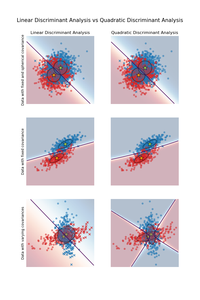
The plot shows decision boundaries for Linear Discriminant Analysis and Quadratic Discriminant Analysis. The bottom row demonstrates that Linear Discriminant Analysis can only learn linear boundaries, while Quadratic Discriminant Analysis can learn quadratic boundaries and is therefore more flexible.
Examples
Linear and Quadratic Discriminant Analysis with covariance ellipsoid: Comparison of LDA and QDA on synthetic data.
1.2.1. Dimensionality reduction using Linear Discriminant Analysis#
LinearDiscriminantAnalysis can be used to
perform supervised dimensionality reduction, by projecting the input data to a
linear subspace consisting of the directions which maximize the separation
between classes (in a precise sense discussed in the mathematics section
below). The dimension of the output is necessarily less than the number of
classes, so this is in general a rather strong dimensionality reduction, and
only makes sense in a multiclass setting.
This is implemented in the transform method. The desired dimensionality can
be set using the n_components parameter. This parameter has no influence
on the fit and predict methods.
Examples
Comparison of LDA and PCA 2D projection of Iris dataset: Comparison of LDA and PCA for dimensionality reduction of the Iris dataset
1.2.2. Mathematical formulation of the LDA and QDA classifiers#
Both LDA and QDA can be derived from simple probabilistic models which model the class conditional distribution of the data \(P(X|y=k)\) for each class \(k\). Predictions can then be obtained by using Bayes’ rule, for each training sample \(x \in \mathbb{R}^d\):
and we select the class \(k\) which maximizes this posterior probability.
More specifically, for linear and quadratic discriminant analysis, \(P(x|y)\) is modeled as a multivariate Gaussian distribution with density:
where \(d\) is the number of features.
1.2.2.1. QDA#
According to the model above, the log of the posterior is:
where the constant term \(Cst\) corresponds to the denominator \(P(x)\), in addition to other constant terms from the Gaussian. The predicted class is the one that maximises this log-posterior.
Note
Relation with Gaussian Naive Bayes
If in the QDA model one assumes that the covariance matrices are diagonal,
then the inputs are assumed to be conditionally independent in each class,
and the resulting classifier is equivalent to the Gaussian Naive Bayes
classifier naive_bayes.GaussianNB.
1.2.2.2. LDA#
LDA is a special case of QDA, where the Gaussians for each class are assumed to share the same covariance matrix: \(\Sigma_k = \Sigma\) for all \(k\). This reduces the log posterior to:
The term \((x-\mu_k)^T \Sigma^{-1} (x-\mu_k)\) corresponds to the Mahalanobis Distance between the sample \(x\) and the mean \(\mu_k\). The Mahalanobis distance tells how close \(x\) is from \(\mu_k\), while also accounting for the variance of each feature. We can thus interpret LDA as assigning \(x\) to the class whose mean is the closest in terms of Mahalanobis distance, while also accounting for the class prior probabilities.
The log-posterior of LDA can also be written [3] as:
where \(\omega_k = \Sigma^{-1} \mu_k\) and \(\omega_{k0} =
-\frac{1}{2} \mu_k^T\Sigma^{-1}\mu_k + \log P (y = k)\). These quantities
correspond to the coef_ and intercept_ attributes, respectively.
From the above formula, it is clear that LDA has a linear decision surface. In the case of QDA, there are no assumptions on the covariance matrices \(\Sigma_k\) of the Gaussians, leading to quadratic decision surfaces. See [1] for more details.
1.2.3. Mathematical formulation of LDA dimensionality reduction#
First note that the K means \(\mu_k\) are vectors in \(\mathbb{R}^d\), and they lie in an affine subspace \(H\) of dimension at most \(K - 1\) (2 points lie on a line, 3 points lie on a plane, etc.).
As mentioned above, we can interpret LDA as assigning \(x\) to the class whose mean \(\mu_k\) is the closest in terms of Mahalanobis distance, while also accounting for the class prior probabilities. Alternatively, LDA is equivalent to first sphering the data so that the covariance matrix is the identity, and then assigning \(x\) to the closest mean in terms of Euclidean distance (still accounting for the class priors).
Computing Euclidean distances in this d-dimensional space is equivalent to first projecting the data points into \(H\), and computing the distances there (since the other dimensions will contribute equally to each class in terms of distance). In other words, if \(x\) is closest to \(\mu_k\) in the original space, it will also be the case in \(H\). This shows that, implicit in the LDA classifier, there is a dimensionality reduction by linear projection onto a \(K-1\) dimensional space.
We can reduce the dimension even more, to a chosen \(L\), by projecting
onto the linear subspace \(H_L\) which maximizes the variance of the
\(\mu^*_k\) after projection (in effect, we are doing a form of PCA for the
transformed class means \(\mu^*_k\)). This \(L\) corresponds to the
n_components parameter used in the
transform method. See
[1] for more details.
1.2.4. Shrinkage and Covariance Estimator#
Shrinkage is a form of regularization used to improve the estimation of
covariance matrices in situations where the number of training samples is
small compared to the number of features.
In this scenario, the empirical sample covariance is a poor
estimator, and shrinkage helps improving the generalization performance of
the classifier.
Shrinkage can be used with LDA (or QDA) by setting the shrinkage parameter of
the LinearDiscriminantAnalysis class
(or QuadraticDiscriminantAnalysis) to 'auto'.
This automatically determines the optimal shrinkage parameter in an analytic
way following the lemma introduced by Ledoit and Wolf [2]. Note that
currently shrinkage only works when setting the solver parameter to 'lsqr'
or 'eigen' (only 'eigen' is implemented for QDA).
The shrinkage parameter can also be manually set between 0 and 1. In
particular, a value of 0 corresponds to no shrinkage (which means the empirical
covariance matrix will be used) and a value of 1 corresponds to complete
shrinkage (which means that the diagonal matrix of variances will be used as
an estimate for the covariance matrix). Setting this parameter to a value
between these two extrema will estimate a shrunk version of the covariance
matrix.
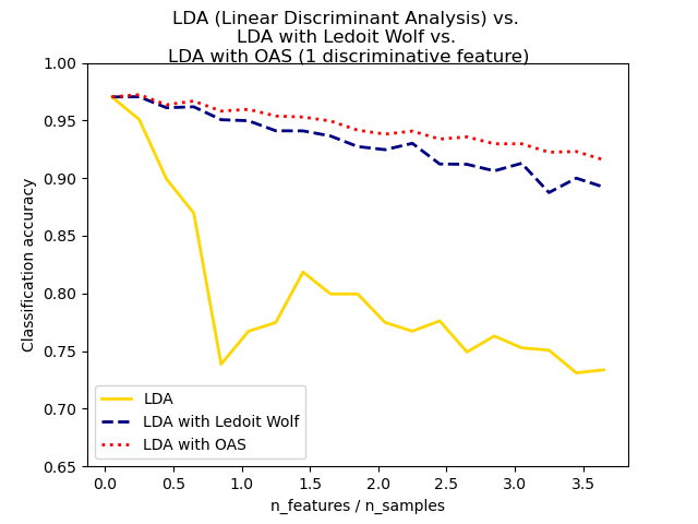
The shrunk Ledoit and Wolf estimator of covariance may not always be the
best choice. For example if the distribution of the data
is normally distributed, the
Oracle Approximating Shrinkage estimator sklearn.covariance.OAS
yields a smaller Mean Squared Error than the one given by Ledoit and Wolf’s
formula used with shrinkage="auto". In LDA and QDA, the data are assumed to be gaussian
conditionally to the class. If these assumptions hold, using LDA and QDA with
the OAS estimator of covariance will yield a better classification
accuracy than if Ledoit and Wolf or the empirical covariance estimator is used.
The covariance estimator can be chosen using the covariance_estimator
parameter of the discriminant_analysis.LinearDiscriminantAnalysis
and discriminant_analysis.QuadraticDiscriminantAnalysis classes.
A covariance estimator should have a fit method and a
covariance_ attribute like all covariance estimators in the
sklearn.covariance module.
Examples
Normal, Ledoit-Wolf and OAS Linear Discriminant Analysis for classification: Comparison of LDA classifiers with Empirical, Ledoit Wolf and OAS covariance estimator.
1.2.5. Estimation algorithms#
Using LDA and QDA requires computing the log-posterior which depends on the class priors \(P(y=k)\), the class means \(\mu_k\), and the covariance matrices.
The ‘svd’ solver is the default solver used for
LinearDiscriminantAnalysis and
QuadraticDiscriminantAnalysis.
It can perform both classification and transform (for LDA).
As it does not rely on the calculation of the covariance matrix, the ‘svd’
solver may be preferable in situations where the number of features is large.
The ‘svd’ solver cannot be used with shrinkage.
For QDA, the use of the SVD solver relies on the fact that the covariance
matrix \(\Sigma_k\) is, by definition, equal to \(\frac{1}{n - 1}
X_k^TX_k = \frac{1}{n - 1} V S^2 V^T\) where \(V\) comes from the SVD of the (centered)
matrix: \(X_k = U S V^T\). It turns out that we can compute the
log-posterior above without having to explicitly compute \(\Sigma\):
computing \(S\) and \(V\) via the SVD of \(X\) is enough. For
LDA, two SVDs are computed: the SVD of the centered input matrix \(X\)
and the SVD of the class-wise mean vectors.
The 'lsqr' solver is an efficient algorithm that only works for
classification. It needs to explicitly compute the covariance matrix
\(\Sigma\), and supports shrinkage and custom covariance estimators.
This solver computes the coefficients
\(\omega_k = \Sigma^{-1}\mu_k\) by solving for \(\Sigma \omega =
\mu_k\), thus avoiding the explicit computation of the inverse
\(\Sigma^{-1}\).
The 'eigen' solver for LinearDiscriminantAnalysis
is based on the optimization of the between class scatter to
within class scatter ratio. It can be used for both classification and
transform, and it supports shrinkage.
For QuadraticDiscriminantAnalysis,
the 'eigen' solver is based on computing the eigenvalues and eigenvectors of each
class covariance matrix. It allows using shrinkage for classification.
However, the 'eigen' solver needs to
compute the covariance matrix, so it might not be suitable for situations with
a high number of features.
References
