1.7. Gaussian Processes#
Gaussian Processes (GP) are a nonparametric supervised learning method used to solve regression and probabilistic classification problems.
The advantages of Gaussian processes are:
The prediction interpolates the observations (at least for regular kernels).
The prediction is probabilistic (Gaussian) so that one can compute empirical confidence intervals and decide based on those if one should refit (online fitting, adaptive fitting) the prediction in some region of interest.
Versatile: different kernels can be specified. Common kernels are provided, but it is also possible to specify custom kernels.
The disadvantages of Gaussian processes include:
Our implementation is not sparse, i.e., they use the whole samples/features information to perform the prediction.
They lose efficiency in high dimensional spaces – namely when the number of features exceeds a few dozens.
1.7.1. Gaussian Process Regression (GPR)#
The GaussianProcessRegressor implements Gaussian processes (GP) for
regression purposes. For this, the prior of the GP needs to be specified. GP
will combine this prior and the likelihood function based on training samples.
It allows to give a probabilistic approach to prediction by giving the mean and
standard deviation as output when predicting.
The prior mean is assumed to be constant and zero (for normalize_y=False) or
the training data’s mean (for normalize_y=True). The prior’s covariance is
specified by passing a kernel object. The hyperparameters
of the kernel are optimized when fitting the GaussianProcessRegressor
by maximizing the log-marginal-likelihood (LML) based on the passed
optimizer. As the LML may have multiple local optima, the optimizer can be
started repeatedly by specifying n_restarts_optimizer. The first run is
always conducted starting from the initial hyperparameter values of the kernel;
subsequent runs are conducted from hyperparameter values that have been chosen
randomly from the range of allowed values. If the initial hyperparameters
should be kept fixed, None can be passed as optimizer.
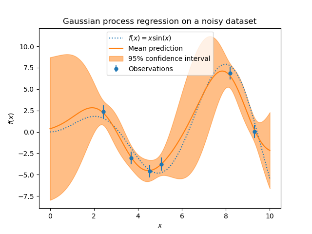
The noise level in the targets can be specified by passing it via the parameter
alpha, either globally as a scalar or per datapoint. Note that a moderate
noise level can also be helpful for dealing with numeric instabilities during
fitting as it is effectively implemented as Tikhonov regularization, i.e., by
adding it to the diagonal of the kernel matrix. An alternative to specifying
the noise level explicitly is to include a
WhiteKernel component into the
kernel, which can estimate the global noise level from the data (see example
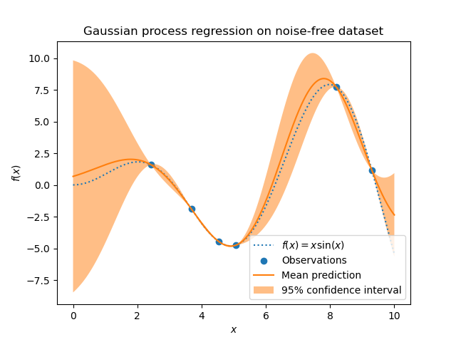
below). The figure below shows the effect of noisy target handled by setting
the parameter alpha.
The implementation is based on Algorithm 2.1 of [RW2006]. In addition to
the API of standard scikit-learn estimators, GaussianProcessRegressor:
allows prediction without prior fitting (based on the GP prior)
provides an additional method
sample_y(X), which evaluates samples drawn from the GPR (prior or posterior) at given inputsexposes a method
log_marginal_likelihood(theta), which can be used externally for other ways of selecting hyperparameters, e.g., via Markov chain Monte Carlo.
Examples
1.7.2. Gaussian Process Classification (GPC)#
The GaussianProcessClassifier implements Gaussian processes (GP) for
classification purposes, more specifically for probabilistic classification,
where test predictions take the form of class probabilities.
GaussianProcessClassifier places a GP prior on a latent function \(f\),
which is then squashed through a link function \(\pi\) to obtain the probabilistic
classification. The latent function \(f\) is a so-called nuisance function,
whose values are not observed and are not relevant by themselves.
Its purpose is to allow a convenient formulation of the model, and \(f\)
is removed (integrated out) during prediction. GaussianProcessClassifier
implements the logistic link function, for which the integral cannot be
computed analytically but is easily approximated in the binary case.
In contrast to the regression setting, the posterior of the latent function \(f\) is not Gaussian even for a GP prior since a Gaussian likelihood is inappropriate for discrete class labels. Rather, a non-Gaussian likelihood corresponding to the logistic link function (logit) is used. GaussianProcessClassifier approximates the non-Gaussian posterior with a Gaussian based on the Laplace approximation. More details can be found in Chapter 3 of [RW2006].
The GP prior mean is assumed to be zero. The prior’s
covariance is specified by passing a kernel object. The
hyperparameters of the kernel are optimized during fitting of
GaussianProcessRegressor by maximizing the log-marginal-likelihood (LML) based
on the passed optimizer. As the LML may have multiple local optima, the
optimizer can be started repeatedly by specifying n_restarts_optimizer. The
first run is always conducted starting from the initial hyperparameter values
of the kernel; subsequent runs are conducted from hyperparameter values
that have been chosen randomly from the range of allowed values.
If the initial hyperparameters should be kept fixed, None can be passed as
optimizer.
In some scenarios, information about the latent function \(f\) is desired
(i.e. the mean \(\bar{f_*}\) and the variance \(\text{Var}[f_*]\) described
in Eqs. (3.21) and (3.24) of [RW2006]). The GaussianProcessClassifier
provides access to these quantities via the latent_mean_and_variance method.
GaussianProcessClassifier supports multi-class classification
by performing either one-versus-rest or one-versus-one based training and
prediction. In one-versus-rest, one binary Gaussian process classifier is
fitted for each class, which is trained to separate this class from the rest.
In “one_vs_one”, one binary Gaussian process classifier is fitted for each pair
of classes, which is trained to separate these two classes. The predictions of
these binary predictors are combined into multi-class predictions. See the
section on multi-class classification for more details.
In the case of Gaussian process classification, “one_vs_one” might be
computationally cheaper since it has to solve many problems involving only a
subset of the whole training set rather than fewer problems on the whole
dataset. Since Gaussian process classification scales cubically with the size
of the dataset, this might be considerably faster. However, note that
“one_vs_one” does not support predicting probability estimates but only plain
predictions. Moreover, note that GaussianProcessClassifier does not
(yet) implement a true multi-class Laplace approximation internally, but
as discussed above is based on solving several binary classification tasks
internally, which are combined using one-versus-rest or one-versus-one.
1.7.3. GPC examples#
1.7.3.1. Probabilistic predictions with GPC#
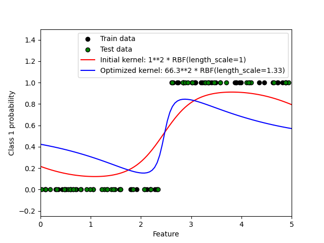
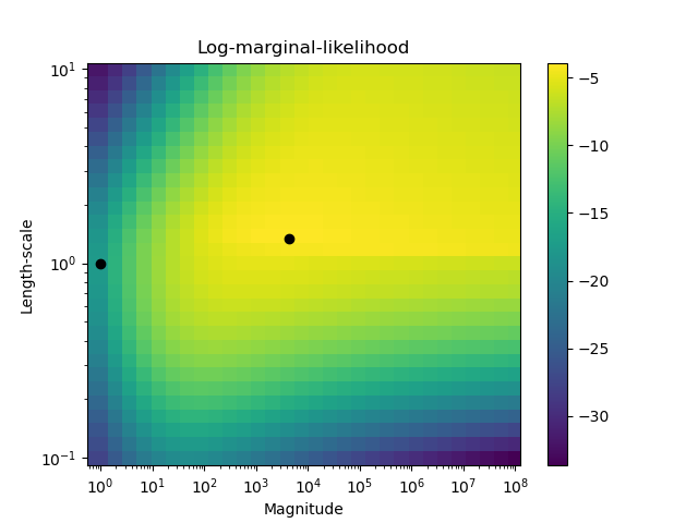
This example illustrates the predicted probability of GPC for an RBF kernel with different choices of the hyperparameters. The first figure shows the predicted probability of GPC with arbitrarily chosen hyperparameters and with the hyperparameters corresponding to the maximum log-marginal-likelihood (LML).
While the hyperparameters chosen by optimizing LML have a considerably larger LML, they perform slightly worse according to the log-loss on test data. The figure shows that this is because they exhibit a steep change of the class probabilities at the class boundaries (which is good) but have predicted probabilities close to 0.5 far away from the class boundaries (which is bad). This undesirable effect is caused by the Laplace approximation used internally by GPC.
The second figure shows the log-marginal-likelihood for different choices of the kernel’s hyperparameters, highlighting the two choices of the hyperparameters used in the first figure by black dots.
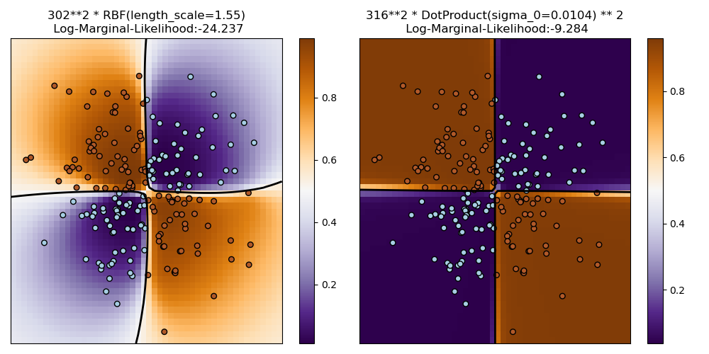
1.7.3.2. Illustration of GPC on the XOR dataset#
This example illustrates GPC on XOR data. Compared are a stationary, isotropic
kernel (RBF) and a non-stationary kernel (DotProduct). On
this particular dataset, the DotProduct kernel obtains considerably
better results because the class-boundaries are linear and coincide with the
coordinate axes. In practice, however, stationary kernels such as RBF
often obtain better results.
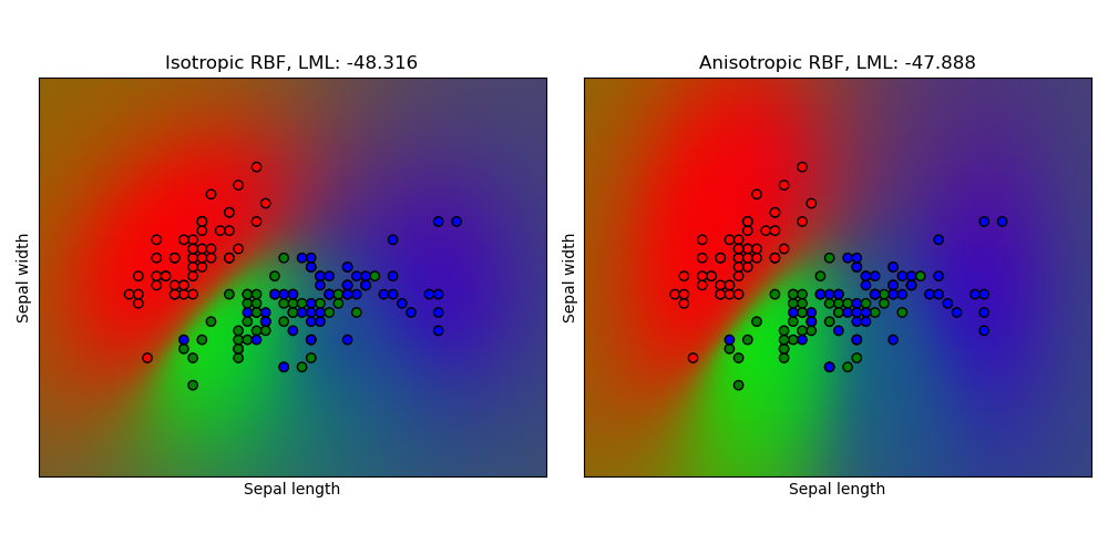
1.7.3.3. Gaussian process classification (GPC) on iris dataset#
This example illustrates the predicted probability of GPC for an isotropic and anisotropic RBF kernel on a two-dimensional version for the iris dataset. This illustrates the applicability of GPC to non-binary classification. The anisotropic RBF kernel obtains slightly higher log-marginal-likelihood by assigning different length-scales to the two feature dimensions.
1.7.4. Kernels for Gaussian Processes#
Kernels (also called “covariance functions” in the context of GPs) are a crucial ingredient of GPs which determine the shape of prior and posterior of the GP. They encode the assumptions on the function being learned by defining the “similarity” of two datapoints combined with the assumption that similar datapoints should have similar target values. Two categories of kernels can be distinguished: stationary kernels depend only on the distance of two datapoints and not on their absolute values \(k(x_i, x_j)= k(d(x_i, x_j))\) and are thus invariant to translations in the input space, while non-stationary kernels depend also on the specific values of the datapoints. Stationary kernels can further be subdivided into isotropic and anisotropic kernels, where isotropic kernels are also invariant to rotations in the input space. For more details, we refer to Chapter 4 of [RW2006]. This example shows how to define a custom kernel over discrete data. For guidance on how to best combine different kernels, we refer to [Duv2014].
Gaussian Process Kernel API#
The main usage of a Kernel is to compute the GP’s covariance between
datapoints. For this, the method __call__ of the kernel can be called. This
method can either be used to compute the “auto-covariance” of all pairs of
datapoints in a 2d array X, or the “cross-covariance” of all combinations
of datapoints of a 2d array X with datapoints in a 2d array Y. The following
identity holds true for all kernels k (except for the WhiteKernel):
k(X) == K(X, Y=X)
If only the diagonal of the auto-covariance is being used, the method diag()
of a kernel can be called, which is more computationally efficient than the
equivalent call to __call__: np.diag(k(X, X)) == k.diag(X)
Kernels are parameterized by a vector \(\theta\) of hyperparameters. These
hyperparameters can for instance control length-scales or periodicity of a
kernel (see below). All kernels support computing analytic gradients
of the kernel’s auto-covariance with respect to \(log(\theta)\) via setting
eval_gradient=True in the __call__ method.
That is, a (len(X), len(X), len(theta)) array is returned where the entry
[i, j, l] contains \(\frac{\partial k_\theta(x_i, x_j)}{\partial log(\theta_l)}\).
This gradient is used by the Gaussian process (both regressor and classifier)
in computing the gradient of the log-marginal-likelihood, which in turn is used
to determine the value of \(\theta\), which maximizes the log-marginal-likelihood,
via gradient ascent. For each hyperparameter, the initial value and the
bounds need to be specified when creating an instance of the kernel. The
current value of \(\theta\) can be get and set via the property
theta of the kernel object. Moreover, the bounds of the hyperparameters can be
accessed by the property bounds of the kernel. Note that both properties
(theta and bounds) return log-transformed values of the internally used values
since those are typically more amenable to gradient-based optimization.
The specification of each hyperparameter is stored in the form of an instance of
Hyperparameter in the respective kernel. Note that a kernel using a
hyperparameter with name “x” must have the attributes self.x and self.x_bounds.
The abstract base class for all kernels is Kernel. Kernel implements a
similar interface as BaseEstimator, providing the
methods get_params(), set_params(), and clone(). This allows
setting kernel values also via meta-estimators such as
Pipeline or
GridSearchCV. Note that due to the nested
structure of kernels (by applying kernel operators, see below), the names of
kernel parameters might become relatively complicated. In general, for a binary
kernel operator, parameters of the left operand are prefixed with k1__ and
parameters of the right operand with k2__. An additional convenience method
is clone_with_theta(theta), which returns a cloned version of the kernel
but with the hyperparameters set to theta. An illustrative example:
>>> from sklearn.gaussian_process.kernels import ConstantKernel, RBF
>>> kernel = ConstantKernel(constant_value=1.0, constant_value_bounds=(0.0, 10.0)) * RBF(length_scale=0.5, length_scale_bounds=(0.0, 10.0)) + RBF(length_scale=2.0, length_scale_bounds=(0.0, 10.0))
>>> for hyperparameter in kernel.hyperparameters: print(hyperparameter)
Hyperparameter(name='k1__k1__constant_value', value_type='numeric', bounds=array([[ 0., 10.]]), n_elements=1, fixed=False)
Hyperparameter(name='k1__k2__length_scale', value_type='numeric', bounds=array([[ 0., 10.]]), n_elements=1, fixed=False)
Hyperparameter(name='k2__length_scale', value_type='numeric', bounds=array([[ 0., 10.]]), n_elements=1, fixed=False)
>>> params = kernel.get_params()
>>> for key in sorted(params): print("%s : %s" % (key, params[key]))
k1 : 1**2 * RBF(length_scale=0.5)
k1__k1 : 1**2
k1__k1__constant_value : 1.0
k1__k1__constant_value_bounds : (0.0, 10.0)
k1__k2 : RBF(length_scale=0.5)
k1__k2__length_scale : 0.5
k1__k2__length_scale_bounds : (0.0, 10.0)
k2 : RBF(length_scale=2)
k2__length_scale : 2.0
k2__length_scale_bounds : (0.0, 10.0)
>>> print(kernel.theta)  # Note: log-transformed
[ 0.         -0.69314718  0.69314718]
>>> print(kernel.bounds)  # Note: log-transformed
[[      -inf 2.30258509]
[      -inf 2.30258509]
[      -inf 2.30258509]]
All Gaussian process kernels are interoperable with sklearn.metrics.pairwise
and vice versa: instances of subclasses of Kernel can be passed as
metric to pairwise_kernels from sklearn.metrics.pairwise. Moreover,
kernel functions from pairwise can be used as GP kernels by using the wrapper
class PairwiseKernel. The only caveat is that the gradient of
the hyperparameters is not analytic but numeric and all those kernels support
only isotropic distances. The parameter gamma is considered to be a
hyperparameter and may be optimized. The other kernel parameters are set
directly at initialization and are kept fixed.
1.7.4.1. Basic kernels#
The ConstantKernel kernel can be used as part of a Product
kernel where it scales the magnitude of the other factor (kernel) or as part
of a Sum kernel, where it modifies the mean of the Gaussian process.
It depends on a parameter \(constant\_value\). It is defined as:
The main use-case of the WhiteKernel kernel is as part of a
sum-kernel where it explains the noise-component of the signal. Tuning its
parameter \(noise\_level\) corresponds to estimating the noise-level.
It is defined as:
1.7.4.2. Kernel operators#
Kernel operators take one or two base kernels and combine them into a new
kernel. The Sum kernel takes two kernels \(k_1\) and \(k_2\)
and combines them via \(k_{sum}(X, Y) = k_1(X, Y) + k_2(X, Y)\).
The Product kernel takes two kernels \(k_1\) and \(k_2\)
and combines them via \(k_{product}(X, Y) = k_1(X, Y) * k_2(X, Y)\).
The Exponentiation kernel takes one base kernel and a scalar parameter
\(p\) and combines them via
\(k_{exp}(X, Y) = k(X, Y)^p\).
Note that magic methods __add__, __mul___ and __pow__ are
overridden on the Kernel objects, so one can use e.g. RBF() + RBF() as
a shortcut for Sum(RBF(), RBF()).
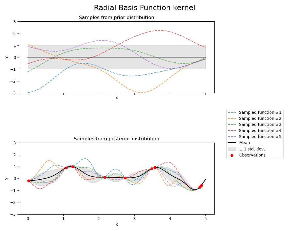
1.7.4.3. Radial basis function (RBF) kernel#
The RBF kernel is a stationary kernel. It is also known as the “squared
exponential” kernel. It is parameterized by a length-scale parameter \(l>0\), which
can either be a scalar (isotropic variant of the kernel) or a vector with the same
number of dimensions as the inputs \(x\) (anisotropic variant of the kernel).
The kernel is given by:
where \(d(\cdot, \cdot)\) is the Euclidean distance. This kernel is infinitely differentiable, which implies that GPs with this kernel as covariance function have mean square derivatives of all orders, and are thus very smooth. The prior and posterior of a GP resulting from an RBF kernel are shown in the following figure:
1.7.4.4. Matérn kernel#
The Matern kernel is a stationary kernel and a generalization of the
RBF kernel. It has an additional parameter \(\nu\) which controls
the smoothness of the resulting function. It is parameterized by a length-scale parameter \(l>0\), which can either be a scalar (isotropic variant of the kernel) or a vector with the same number of dimensions as the inputs \(x\) (anisotropic variant of the kernel).
Mathematical implementation of Matérn kernel#
The kernel is given by:
where \(d(\cdot,\cdot)\) is the Euclidean distance, \(K_\nu(\cdot)\) is a modified Bessel function and \(\Gamma(\cdot)\) is the gamma function. As \(\nu\rightarrow\infty\), the Matérn kernel converges to the RBF kernel. When \(\nu = 1/2\), the Matérn kernel becomes identical to the absolute exponential kernel, i.e.,
In particular, \(\nu = 3/2\):
and \(\nu = 5/2\):
are popular choices for learning functions that are not infinitely differentiable (as assumed by the RBF kernel) but at least once (\(\nu = 3/2\)) or twice differentiable (\(\nu = 5/2\)).
The flexibility of controlling the smoothness of the learned function via \(\nu\) allows adapting to the properties of the true underlying functional relation.
The prior and posterior of a GP resulting from a Matérn kernel are shown in the following figure:
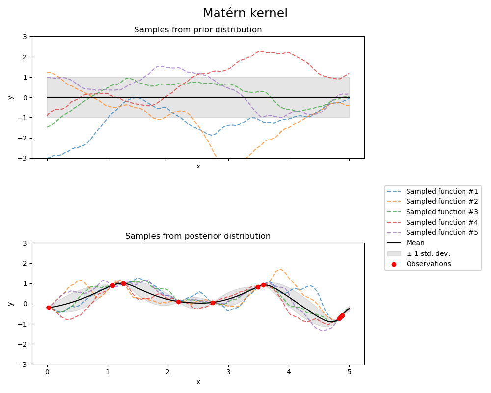
See [RW2006], pp84 for further details regarding the different variants of the Matérn kernel.
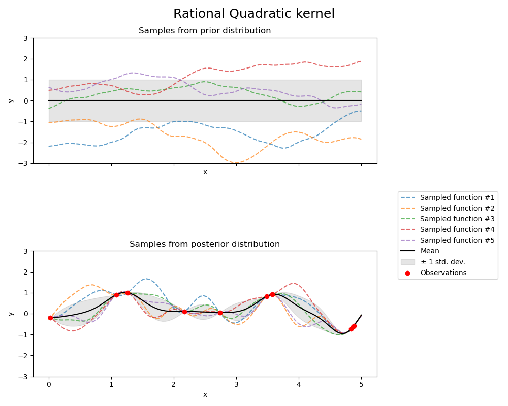
1.7.4.5. Rational quadratic kernel#
The RationalQuadratic kernel can be seen as a scale mixture (an infinite sum)
of RBF kernels with different characteristic length-scales. It is parameterized
by a length-scale parameter \(l>0\) and a scale mixture parameter \(\alpha>0\)
Only the isotropic variant where \(l\) is a scalar is supported at the moment.
The kernel is given by:
The prior and posterior of a GP resulting from a RationalQuadratic kernel are shown in
the following figure:
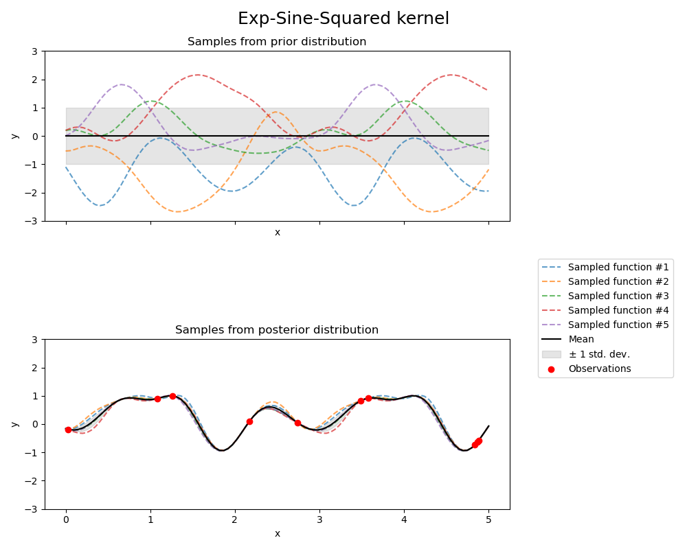
1.7.4.6. Exp-Sine-Squared kernel#
The ExpSineSquared kernel allows modeling periodic functions.
It is parameterized by a length-scale parameter \(l>0\) and a periodicity parameter
\(p>0\). Only the isotropic variant where \(l\) is a scalar is supported at the moment.
The kernel is given by:
The prior and posterior of a GP resulting from an ExpSineSquared kernel are shown in the following figure:
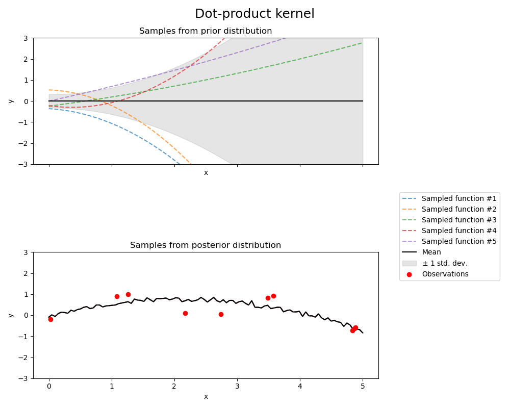
1.7.4.7. Dot-Product kernel#
The DotProduct kernel is non-stationary and can be obtained from linear regression
by putting \(N(0, 1)\) priors on the coefficients of \(x_d (d = 1, . . . , D)\) and
a prior of \(N(0, \sigma_0^2)\) on the bias. The DotProduct kernel is invariant to a rotation
of the coordinates about the origin, but not translations.
It is parameterized by a parameter \(\sigma_0^2\). For \(\sigma_0^2 = 0\), the kernel
is called the homogeneous linear kernel, otherwise it is inhomogeneous. The kernel is given by
The DotProduct kernel is commonly combined with exponentiation. An example with exponent 2 is
shown in the following figure: