5.1. Partial Dependence and Individual Conditional Expectation plots#
Partial dependence plots (PDP) and individual conditional expectation (ICE) plots can be used to visualize and analyze interaction between the target response [1] and a set of input features of interest.
Both PDPs [H2009] and ICEs [G2015] assume that the input features of interest are independent from the complement features, and this assumption is often violated in practice. Thus, in the case of correlated features, we will create absurd data points to compute the PDP/ICE [M2019].
5.1.1. Partial dependence plots#
Partial dependence plots (PDP) show the dependence between the target response and a set of input features of interest, marginalizing over the values of all other input features (the ‘complement’ features). Intuitively, we can interpret the partial dependence as the expected target response as a function of the input features of interest.
Due to the limits of human perception, the size of the set of input features of interest must be small (usually, one or two) thus the input features of interest are usually chosen among the most important features.
The figure below shows two one-way and one two-way partial dependence plots for
the bike sharing dataset, with a
HistGradientBoostingRegressor:
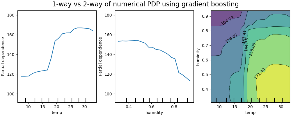
One-way PDPs tell us about the interaction between the target response and an input feature of interest (e.g. linear, non-linear). The left plot in the above figure shows the effect of the temperature on the number of bike rentals; we can clearly see that a higher temperature is related with a higher number of bike rentals. Similarly, we could analyze the effect of the humidity on the number of bike rentals (middle plot). Thus, these interpretations are marginal, considering a feature at a time.
PDPs with two input features of interest show the interactions among the two features. For example, the two-variable PDP in the above figure shows the dependence of the number of bike rentals on joint values of temperature and humidity. We can clearly see an interaction between the two features: with a temperature higher than 20 degrees Celsius, mainly the humidity has a strong impact on the number of bike rentals. For lower temperatures, both the temperature and the humidity have an impact on the number of bike rentals.
The sklearn.inspection module provides a convenience function
from_estimator to create one-way and two-way partial
dependence plots. In the below example we show how to create a grid of
partial dependence plots: two one-way PDPs for the features 0 and 1
and a two-way PDP between the two features:
>>> from sklearn.datasets import make_hastie_10_2
>>> from sklearn.ensemble import GradientBoostingClassifier
>>> from sklearn.inspection import PartialDependenceDisplay

>>> X, y = make_hastie_10_2(random_state=0)
>>> clf = GradientBoostingClassifier(n_estimators=100, learning_rate=1.0,
...     max_depth=1, random_state=0).fit(X, y)
>>> features = [0, 1, (0, 1)]
>>> PartialDependenceDisplay.from_estimator(clf, X, features)
<...>
You can access the newly created figure and Axes objects using plt.gcf()
and plt.gca().
To make a partial dependence plot with categorical features, you need to specify
which features are categorical using the parameter categorical_features. This
parameter takes a list of indices, names of the categorical features or a boolean
mask. The graphical representation of partial dependence for categorical features is
a bar plot or a 2D heatmap.
PDPs for multi-class classification#
For multi-class classification, you need to set the class label for which
the PDPs should be created via the target argument:
>>> from sklearn.datasets import load_iris
>>> iris = load_iris()
>>> mc_clf = GradientBoostingClassifier(n_estimators=10,
...     max_depth=1).fit(iris.data, iris.target)
>>> features = [3, 2, (3, 2)]
>>> PartialDependenceDisplay.from_estimator(mc_clf, X, features, target=0)
<...>
The same parameter target is used to specify the target in multi-output
regression settings.
If you need the raw values of the partial dependence function rather than
the plots, you can use the
sklearn.inspection.partial_dependence function:
>>> from sklearn.inspection import partial_dependence

>>> results = partial_dependence(clf, X, [0])
>>> results["average"]
array([[ 2.466...,  2.466..., ...
>>> results["grid_values"]
[array([-1.624..., -1.592..., ...
The values at which the partial dependence should be evaluated are directly
generated from X. For 2-way partial dependence, a 2D-grid of values is
generated. The values field returned by
sklearn.inspection.partial_dependence gives the actual values
used in the grid for each input feature of interest. They also correspond to
the axis of the plots.
5.1.2. Individual conditional expectation (ICE) plot#
Similar to a PDP, an individual conditional expectation (ICE) plot shows the dependence between the target function and an input feature of interest. However, unlike a PDP, which shows the average effect of the input feature, an ICE plot visualizes the dependence of the prediction on a feature for each sample separately with one line per sample. Due to the limits of human perception, only one input feature of interest is supported for ICE plots.
The figures below show two ICE plots for the bike sharing dataset,
with a HistGradientBoostingRegressor. The figures plot
the corresponding PD line overlaid on ICE lines.
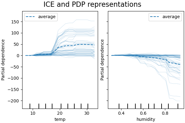
While the PDPs are good at showing the average effect of the target features, they can obscure a heterogeneous relationship created by interactions. When interactions are present the ICE plot will provide many more insights. For example, we see that the ICE for the temperature feature gives us some additional information: some of the ICE lines are flat while some others show a decrease of the dependence for temperature above 35 degrees Celsius. We observe a similar pattern for the humidity feature: some of the ICE lines show a sharp decrease when the humidity is above 80%.
The sklearn.inspection module’s PartialDependenceDisplay.from_estimator
convenience function can be used to create ICE plots by setting
kind='individual'. In the example below, we show how to create a grid of
ICE plots:
>>> from sklearn.datasets import make_hastie_10_2
>>> from sklearn.ensemble import GradientBoostingClassifier
>>> from sklearn.inspection import PartialDependenceDisplay
>>> X, y = make_hastie_10_2(random_state=0)
>>> clf = GradientBoostingClassifier(n_estimators=100, learning_rate=1.0,
...     max_depth=1, random_state=0).fit(X, y)
>>> features = [0, 1]
>>> PartialDependenceDisplay.from_estimator(clf, X, features,
...     kind='individual')
<...>
In ICE plots it might not be easy to see the average effect of the input
feature of interest. Hence, it is recommended to use ICE plots alongside
PDPs. They can be plotted together with
kind='both'.
>>> PartialDependenceDisplay.from_estimator(clf, X, features,
...     kind='both')
<...>
If there are too many lines in an ICE plot, it can be difficult to see
differences between individual samples and interpret the model. Centering the
ICE at the first value on the x-axis, produces centered Individual Conditional
Expectation (cICE) plots [G2015]. This puts emphasis on the divergence of
individual conditional expectations from the mean line, thus making it easier
to explore heterogeneous relationships. cICE plots can be plotted by setting
centered=True:
>>> PartialDependenceDisplay.from_estimator(clf, X, features,
...     kind='both', centered=True)
<...>
5.1.3. Mathematical Definition#
Let \(X_S\) be the set of input features of interest (i.e. the features
parameter) and let \(X_C\) be its complement.
The partial dependence of the response \(f\) at a point \(x_S\) is defined as:
where \(f(x_S, x_C)\) is the response function (predict, predict_proba or decision_function) for a given sample whose values are defined by \(x_S\) for the features in \(X_S\), and by \(x_C\) for the features in \(X_C\). Note that \(x_S\) and \(x_C\) may be tuples.
Computing this integral for various values of \(x_S\) produces a PDP plot as above. An ICE line is defined as a single \(f(x_{S}, x_{C}^{(i)})\) evaluated at \(x_{S}\).
5.1.4. Computation methods#
There are two main methods to approximate the integral above, namely the
'brute' and 'recursion' methods. The method parameter controls which method
to use.
The 'brute' method is a generic method that works with any estimator. Note that
computing ICE plots is only supported with the 'brute' method. It
approximates the above integral by computing an average over the data X:
where \(x_C^{(i)}\) is the value of the i-th sample for the features in
\(X_C\). For each value of \(x_S\), this method requires a full pass
over the dataset X which is computationally intensive.
Each of the \(f(x_{S}, x_{C}^{(i)})\) corresponds to one ICE line evaluated at \(x_{S}\). Computing this for multiple values of \(x_{S}\), one obtains a full ICE line. As one can see, the average of the ICE lines corresponds to the partial dependence line.
The 'recursion' method is faster than the 'brute' method, but it is only
supported for PDP plots by some tree-based estimators. It is computed as
follows. For a given point \(x_S\), a weighted tree traversal is performed:
if a split node involves an input feature of interest, the corresponding left
or right branch is followed; otherwise both branches are followed, each branch
being weighted by the fraction of training samples that entered that branch.
Finally, the partial dependence is given by a weighted average of all the
visited leaves’ values.
With the 'brute' method, the parameter X is used both for generating the
grid of values \(x_S\) and the complement feature values \(x_C\).
However with the ‘recursion’ method, X is only used for the grid values:
implicitly, the \(x_C\) values are those of the training data.
By default, the 'recursion' method is used for plotting PDPs on tree-based
estimators that support it, and ‘brute’ is used for the rest.
Note
While both methods should be close in general, they might differ in some
specific settings. The 'brute' method assumes the existence of the
data points \((x_S, x_C^{(i)})\). When the features are correlated,
such artificial samples may have a very low probability mass. The 'brute'
and 'recursion' methods will likely disagree regarding the value of the
partial dependence, because they will treat these unlikely
samples differently. Remember, however, that the primary assumption for
interpreting PDPs is that the features should be independent.
Examples
Footnotes
References
T. Hastie, R. Tibshirani and J. Friedman, The Elements of Statistical Learning, Second Edition, Section 10.13.2, Springer, 2009.
C. Molnar, Interpretable Machine Learning, Section 5.1, 2019.
