Demo of affinity propagation clustering algorithm#
Reference: Brendan J. Frey and Delbert Dueck, “Clustering by Passing Messages Between Data Points”, Science Feb. 2007
import numpy as np

from sklearn import metrics
from sklearn.cluster import AffinityPropagation
from sklearn.datasets import make_blobs
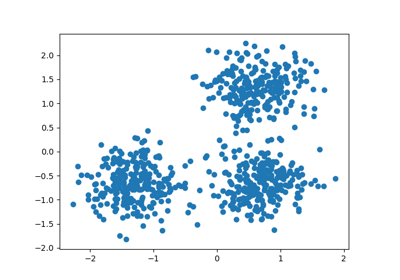
Generate sample data#
centers = [[1, 1], [-1, -1], [1, -1]]
X, labels_true = make_blobs(
    n_samples=300, centers=centers, cluster_std=0.5, random_state=0
)
Compute Affinity Propagation#
af = AffinityPropagation(preference=-50, random_state=0).fit(X)
cluster_centers_indices = af.cluster_centers_indices_
labels = af.labels_

n_clusters_ = len(cluster_centers_indices)

print("Estimated number of clusters: %d" % n_clusters_)
print("Homogeneity: %0.3f" % metrics.homogeneity_score(labels_true, labels))
print("Completeness: %0.3f" % metrics.completeness_score(labels_true, labels))
print("V-measure: %0.3f" % metrics.v_measure_score(labels_true, labels))
print("Adjusted Rand Index: %0.3f" % metrics.adjusted_rand_score(labels_true, labels))
print(
    "Adjusted Mutual Information: %0.3f"
    % metrics.adjusted_mutual_info_score(labels_true, labels)
)
print(
    "Silhouette Coefficient: %0.3f"
    % metrics.silhouette_score(X, labels, metric="sqeuclidean")
)
Estimated number of clusters: 3
Homogeneity: 0.872
Completeness: 0.872
V-measure: 0.872
Adjusted Rand Index: 0.912
Adjusted Mutual Information: 0.871
Silhouette Coefficient: 0.753
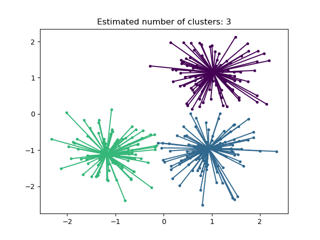
Plot result#
import matplotlib.pyplot as plt

plt.close("all")
plt.figure(1)
plt.clf()

colors = plt.cycler("color", plt.cm.viridis(np.linspace(0, 1, 4)))

for k, col in zip(range(n_clusters_), colors):
    class_members = labels == k
    cluster_center = X[cluster_centers_indices[k]]
    plt.scatter(
        X[class_members, 0], X[class_members, 1], color=col["color"], marker="."
    )
    plt.scatter(
        cluster_center[0], cluster_center[1], s=14, color=col["color"], marker="o"
    )
    for x in X[class_members]:
        plt.plot(
            [cluster_center[0], x[0]], [cluster_center[1], x[1]], color=col["color"]
        )

plt.title("Estimated number of clusters: %d" % n_clusters_)
plt.show()
Total running time of the script: (0 minutes 0.298 seconds)
Related examples
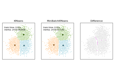
Comparison of the K-Means and MiniBatchKMeans clustering algorithms
Comparison of the K-Means and MiniBatchKMeans clustering algorithms
Adjustment for chance in clustering performance evaluation
Adjustment for chance in clustering performance evaluation