Robust covariance estimation and Mahalanobis distances relevance#
This example shows covariance estimation with Mahalanobis distances on Gaussian distributed data.
For Gaussian distributed data, the distance of an observation \(x_i\) to the mode of the distribution can be computed using its Mahalanobis distance:
where \(\mu\) and \(\Sigma\) are the location and the covariance of the underlying Gaussian distributions.
In practice, \(\mu\) and \(\Sigma\) are replaced by some estimates. The standard covariance maximum likelihood estimate (MLE) is very sensitive to the presence of outliers in the data set and therefore, the downstream Mahalanobis distances also are. It would be better to use a robust estimator of covariance to guarantee that the estimation is resistant to “erroneous” observations in the dataset and that the calculated Mahalanobis distances accurately reflect the true organization of the observations.
The Minimum Covariance Determinant estimator (MCD) is a robust, high-breakdown point (i.e. it can be used to estimate the covariance matrix of highly contaminated datasets, up to \(\frac{n_\text{samples}-n_\text{features}-1}{2}\) outliers) estimator of covariance. The idea behind the MCD is to find \(\frac{n_\text{samples}+n_\text{features}+1}{2}\) observations whose empirical covariance has the smallest determinant, yielding a “pure” subset of observations from which to compute standards estimates of location and covariance. The MCD was introduced by P.J.Rousseuw in [1].
This example illustrates how the Mahalanobis distances are affected by outlying data. Observations drawn from a contaminating distribution are not distinguishable from the observations coming from the real, Gaussian distribution when using standard covariance MLE based Mahalanobis distances. Using MCD-based Mahalanobis distances, the two populations become distinguishable. Associated applications include outlier detection, observation ranking and clustering.
Note
References
Generate data#
First, we generate a dataset of 125 samples and 2 features. Both features are Gaussian distributed with mean of 0 but feature 1 has a standard deviation equal to 2 and feature 2 has a standard deviation equal to 1. Next, 25 samples are replaced with Gaussian outlier samples where feature 1 has a standard deviation equal to 1 and feature 2 has a standard deviation equal to 7.
import numpy as np

# for consistent results
np.random.seed(7)

n_samples = 125
n_outliers = 25
n_features = 2

# generate Gaussian data of shape (125, 2)
gen_cov = np.eye(n_features)
gen_cov[0, 0] = 2.0
X = np.dot(np.random.randn(n_samples, n_features), gen_cov)
# add some outliers
outliers_cov = np.eye(n_features)
outliers_cov[np.arange(1, n_features), np.arange(1, n_features)] = 7.0
X[-n_outliers:] = np.dot(np.random.randn(n_outliers, n_features), outliers_cov)
Comparison of results#
Below, we fit MCD and MLE based covariance estimators to our data and print the estimated covariance matrices. Note that the estimated variance of feature 2 is much higher with the MLE based estimator (7.5) than that of the MCD robust estimator (1.2). This shows that the MCD based robust estimator is much more resistant to the outlier samples, which were designed to have a much larger variance in feature 2.
import matplotlib.pyplot as plt

from sklearn.covariance import EmpiricalCovariance, MinCovDet

# fit a MCD robust estimator to data
robust_cov = MinCovDet().fit(X)
# fit a MLE estimator to data
emp_cov = EmpiricalCovariance().fit(X)
print(
    "Estimated covariance matrix:\nMCD (Robust):\n{}\nMLE:\n{}".format(
        robust_cov.covariance_, emp_cov.covariance_
    )
)
Estimated covariance matrix:
MCD (Robust):
[[ 3.26253567e+00 -3.06695631e-03]
 [-3.06695631e-03  1.22747343e+00]]
MLE:
[[ 3.23773583 -0.24640578]
 [-0.24640578  7.51963999]]
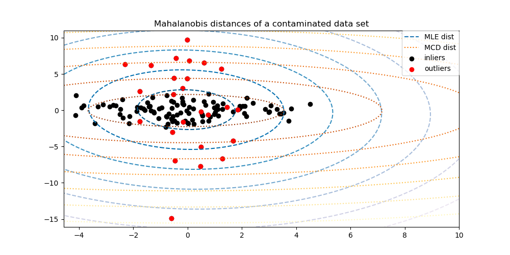
To better visualize the difference, we plot contours of the Mahalanobis distances calculated by both methods. Notice that the robust MCD based Mahalanobis distances fit the inlier black points much better, whereas the MLE based distances are more influenced by the outlier red points.
import matplotlib.lines as mlines

fig, ax = plt.subplots(figsize=(10, 5))
# Plot data set
inlier_plot = ax.scatter(X[:, 0], X[:, 1], color="black", label="inliers")
outlier_plot = ax.scatter(
    X[:, 0][-n_outliers:], X[:, 1][-n_outliers:], color="red", label="outliers"
)
ax.set_xlim(ax.get_xlim()[0], 10.0)
ax.set_title("Mahalanobis distances of a contaminated data set")

# Create meshgrid of feature 1 and feature 2 values
xx, yy = np.meshgrid(
    np.linspace(plt.xlim()[0], plt.xlim()[1], 100),
    np.linspace(plt.ylim()[0], plt.ylim()[1], 100),
)
zz = np.c_[xx.ravel(), yy.ravel()]
# Calculate the MLE based Mahalanobis distances of the meshgrid
mahal_emp_cov = emp_cov.mahalanobis(zz)
mahal_emp_cov = mahal_emp_cov.reshape(xx.shape)
emp_cov_contour = plt.contour(
    xx, yy, np.sqrt(mahal_emp_cov), cmap=plt.cm.PuBu_r, linestyles="dashed"
)
# Calculate the MCD based Mahalanobis distances
mahal_robust_cov = robust_cov.mahalanobis(zz)
mahal_robust_cov = mahal_robust_cov.reshape(xx.shape)
robust_contour = ax.contour(
    xx, yy, np.sqrt(mahal_robust_cov), cmap=plt.cm.YlOrBr_r, linestyles="dotted"
)

# Add legend
ax.legend(
    [
        mlines.Line2D([], [], color="tab:blue", linestyle="dashed"),
        mlines.Line2D([], [], color="tab:orange", linestyle="dotted"),
        inlier_plot,
        outlier_plot,
    ],
    ["MLE dist", "MCD dist", "inliers", "outliers"],
    loc="upper right",
    borderaxespad=0,
)

plt.show()
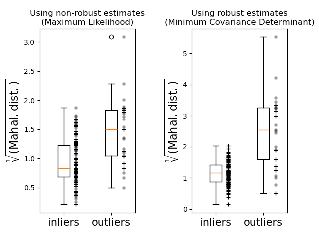
Finally, we highlight the ability of MCD based Mahalanobis distances to distinguish outliers. We take the cubic root of the Mahalanobis distances, yielding approximately normal distributions (as suggested by Wilson and Hilferty [2]), then plot the values of inlier and outlier samples with boxplots. The distribution of outlier samples is more separated from the distribution of inlier samples for robust MCD based Mahalanobis distances.
fig, (ax1, ax2) = plt.subplots(1, 2)
plt.subplots_adjust(wspace=0.6)

# Calculate cubic root of MLE Mahalanobis distances for samples
emp_mahal = emp_cov.mahalanobis(X - np.mean(X, 0)) ** (0.33)
# Plot boxplots
ax1.boxplot([emp_mahal[:-n_outliers], emp_mahal[-n_outliers:]], widths=0.25)
# Plot individual samples
ax1.plot(
    np.full(n_samples - n_outliers, 1.26),
    emp_mahal[:-n_outliers],
    "+k",
    markeredgewidth=1,
)
ax1.plot(np.full(n_outliers, 2.26), emp_mahal[-n_outliers:], "+k", markeredgewidth=1)
ax1.axes.set_xticklabels(("inliers", "outliers"), size=15)
ax1.set_ylabel(r"$\sqrt[3]{\rm{(Mahal. dist.)}}$", size=16)
ax1.set_title("Using non-robust estimates\n(Maximum Likelihood)")

# Calculate cubic root of MCD Mahalanobis distances for samples
robust_mahal = robust_cov.mahalanobis(X - robust_cov.location_) ** (0.33)
# Plot boxplots
ax2.boxplot([robust_mahal[:-n_outliers], robust_mahal[-n_outliers:]], widths=0.25)
# Plot individual samples
ax2.plot(
    np.full(n_samples - n_outliers, 1.26),
    robust_mahal[:-n_outliers],
    "+k",
    markeredgewidth=1,
)
ax2.plot(np.full(n_outliers, 2.26), robust_mahal[-n_outliers:], "+k", markeredgewidth=1)
ax2.axes.set_xticklabels(("inliers", "outliers"), size=15)
ax2.set_ylabel(r"$\sqrt[3]{\rm{(Mahal. dist.)}}$", size=16)
ax2.set_title("Using robust estimates\n(Minimum Covariance Determinant)")

plt.show()
Total running time of the script: (0 minutes 0.283 seconds)
Related examples
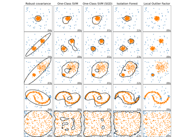
Comparing anomaly detection algorithms for outlier detection on toy datasets
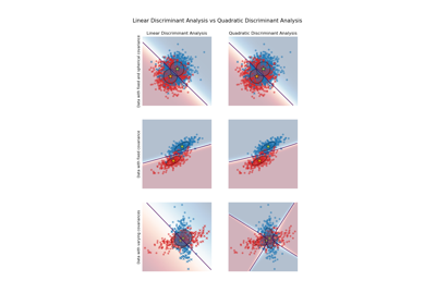
Linear and Quadratic Discriminant Analysis with covariance ellipsoid