Effect of transforming the targets in regression model#
In this example, we give an overview of
TransformedTargetRegressor. We use two examples
to illustrate the benefit of transforming the targets before learning a linear
regression model. The first example uses synthetic data while the second
example is based on the Ames housing data set.
# Author: Guillaume Lemaitre <guillaume.lemaitre@inria.fr>
# License: BSD 3 clause

print(__doc__)
Synthetic example#
A synthetic random regression dataset is generated. The targets
yare modified by:
translating all targets such that all entries are non-negative (by adding the absolute value of the lowest
y) andapplying an exponential function to obtain non-linear targets which cannot be fitted using a simple linear model.
Therefore, a logarithmic (
np.log1p) and an exponential function (np.expm1) will be used to transform the targets before training a linear regression model and using it for prediction.
import numpy as np

from sklearn.datasets import make_regression

X, y = make_regression(n_samples=10_000, noise=100, random_state=0)
y = np.expm1((y + abs(y.min())) / 200)
y_trans = np.log1p(y)
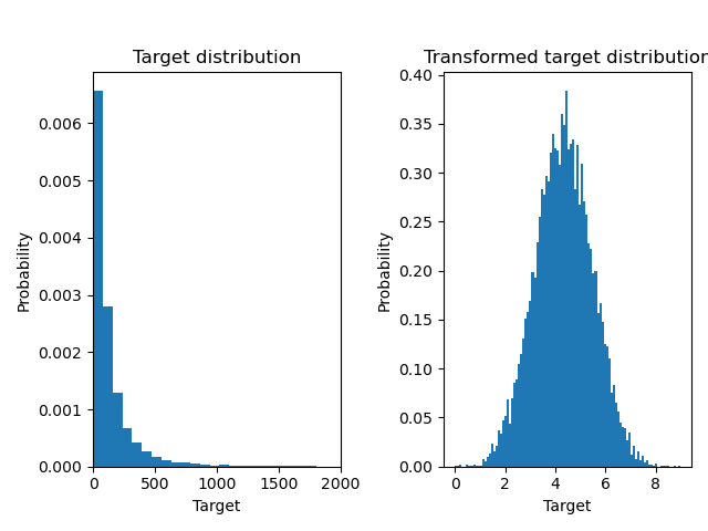
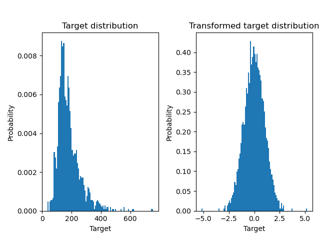
Below we plot the probability density functions of the target before and after applying the logarithmic functions.
import matplotlib.pyplot as plt

from sklearn.model_selection import train_test_split

f, (ax0, ax1) = plt.subplots(1, 2)

ax0.hist(y, bins=100, density=True)
ax0.set_xlim([0, 2000])
ax0.set_ylabel("Probability")
ax0.set_xlabel("Target")
ax0.set_title("Target distribution")

ax1.hist(y_trans, bins=100, density=True)
ax1.set_ylabel("Probability")
ax1.set_xlabel("Target")
ax1.set_title("Transformed target distribution")

f.suptitle("Synthetic data", y=1.05)
plt.tight_layout()

X_train, X_test, y_train, y_test = train_test_split(X, y, random_state=0)
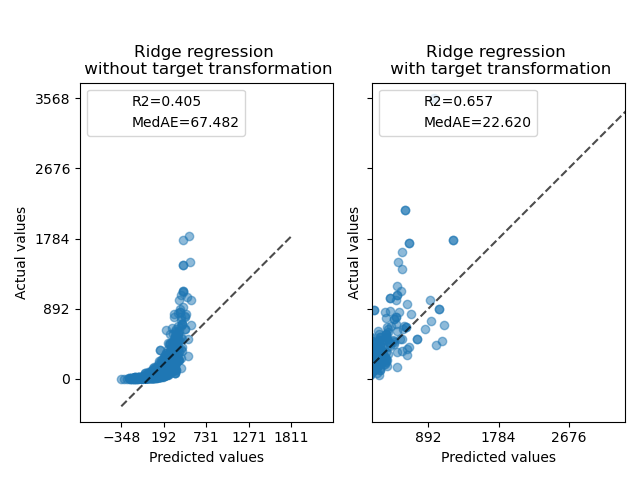
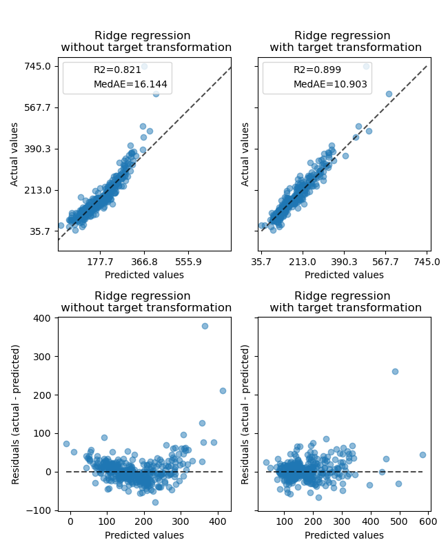
At first, a linear model will be applied on the original targets. Due to the non-linearity, the model trained will not be precise during prediction. Subsequently, a logarithmic function is used to linearize the targets, allowing better prediction even with a similar linear model as reported by the median absolute error (MedAE).
from sklearn.metrics import median_absolute_error, r2_score


def compute_score(y_true, y_pred):
    return {
        "R2": f"{r2_score(y_true, y_pred):.3f}",
        "MedAE": f"{median_absolute_error(y_true, y_pred):.3f}",
    }
from sklearn.compose import TransformedTargetRegressor
from sklearn.linear_model import RidgeCV
from sklearn.metrics import PredictionErrorDisplay

f, (ax0, ax1) = plt.subplots(1, 2, sharey=True)

ridge_cv = RidgeCV().fit(X_train, y_train)
y_pred_ridge = ridge_cv.predict(X_test)

ridge_cv_with_trans_target = TransformedTargetRegressor(
    regressor=RidgeCV(), func=np.log1p, inverse_func=np.expm1
).fit(X_train, y_train)
y_pred_ridge_with_trans_target = ridge_cv_with_trans_target.predict(X_test)

PredictionErrorDisplay.from_predictions(
    y_test,
    y_pred_ridge,
    kind="actual_vs_predicted",
    ax=ax0,
    scatter_kwargs={"alpha": 0.5},
)
PredictionErrorDisplay.from_predictions(
    y_test,
    y_pred_ridge_with_trans_target,
    kind="actual_vs_predicted",
    ax=ax1,
    scatter_kwargs={"alpha": 0.5},
)

# Add the score in the legend of each axis
for ax, y_pred in zip([ax0, ax1], [y_pred_ridge, y_pred_ridge_with_trans_target]):
    for name, score in compute_score(y_test, y_pred).items():
        ax.plot([], [], " ", label=f"{name}={score}")
    ax.legend(loc="upper left")

ax0.set_title("Ridge regression \n without target transformation")
ax1.set_title("Ridge regression \n with target transformation")
f.suptitle("Synthetic data", y=1.05)
plt.tight_layout()
Real-world data set#
In a similar manner, the Ames housing data set is used to show the impact of transforming the targets before learning a model. In this example, the target to be predicted is the selling price of each house.
from sklearn.datasets import fetch_openml
from sklearn.preprocessing import quantile_transform

ames = fetch_openml(name="house_prices", as_frame=True)
# Keep only numeric columns
X = ames.data.select_dtypes(np.number)
# Remove columns with NaN or Inf values
X = X.drop(columns=["LotFrontage", "GarageYrBlt", "MasVnrArea"])
# Let the price be in k$
y = ames.target / 1000
y_trans = quantile_transform(
    y.to_frame(), n_quantiles=900, output_distribution="normal", copy=True
).squeeze()
A QuantileTransformer is used to normalize
the target distribution before applying a
RidgeCV model.
f, (ax0, ax1) = plt.subplots(1, 2)

ax0.hist(y, bins=100, density=True)
ax0.set_ylabel("Probability")
ax0.set_xlabel("Target")
ax0.set_title("Target distribution")

ax1.hist(y_trans, bins=100, density=True)
ax1.set_ylabel("Probability")
ax1.set_xlabel("Target")
ax1.set_title("Transformed target distribution")

f.suptitle("Ames housing data: selling price", y=1.05)
plt.tight_layout()
X_train, X_test, y_train, y_test = train_test_split(X, y, random_state=1)
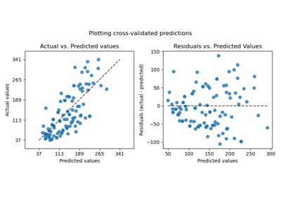
The effect of the transformer is weaker than on the synthetic data. However, the transformation results in an increase in \(R^2\) and large decrease of the MedAE. The residual plot (predicted target - true target vs predicted target) without target transformation takes on a curved, ‘reverse smile’ shape due to residual values that vary depending on the value of predicted target. With target transformation, the shape is more linear indicating better model fit.
from sklearn.preprocessing import QuantileTransformer

f, (ax0, ax1) = plt.subplots(2, 2, sharey="row", figsize=(6.5, 8))

ridge_cv = RidgeCV().fit(X_train, y_train)
y_pred_ridge = ridge_cv.predict(X_test)

ridge_cv_with_trans_target = TransformedTargetRegressor(
    regressor=RidgeCV(),
    transformer=QuantileTransformer(n_quantiles=900, output_distribution="normal"),
).fit(X_train, y_train)
y_pred_ridge_with_trans_target = ridge_cv_with_trans_target.predict(X_test)

# plot the actual vs predicted values
PredictionErrorDisplay.from_predictions(
    y_test,
    y_pred_ridge,
    kind="actual_vs_predicted",
    ax=ax0[0],
    scatter_kwargs={"alpha": 0.5},
)
PredictionErrorDisplay.from_predictions(
    y_test,
    y_pred_ridge_with_trans_target,
    kind="actual_vs_predicted",
    ax=ax0[1],
    scatter_kwargs={"alpha": 0.5},
)

# Add the score in the legend of each axis
for ax, y_pred in zip([ax0[0], ax0[1]], [y_pred_ridge, y_pred_ridge_with_trans_target]):
    for name, score in compute_score(y_test, y_pred).items():
        ax.plot([], [], " ", label=f"{name}={score}")
    ax.legend(loc="upper left")

ax0[0].set_title("Ridge regression \n without target transformation")
ax0[1].set_title("Ridge regression \n with target transformation")

# plot the residuals vs the predicted values
PredictionErrorDisplay.from_predictions(
    y_test,
    y_pred_ridge,
    kind="residual_vs_predicted",
    ax=ax1[0],
    scatter_kwargs={"alpha": 0.5},
)
PredictionErrorDisplay.from_predictions(
    y_test,
    y_pred_ridge_with_trans_target,
    kind="residual_vs_predicted",
    ax=ax1[1],
    scatter_kwargs={"alpha": 0.5},
)
ax1[0].set_title("Ridge regression \n without target transformation")
ax1[1].set_title("Ridge regression \n with target transformation")

f.suptitle("Ames housing data: selling price", y=1.05)
plt.tight_layout()
plt.show()
Total running time of the script: (0 minutes 1.568 seconds)
Related examples
Pipelining: chaining a PCA and a logistic regression