Gradient Boosting regression

This example demonstrates Gradient Boosting to produce a predictive model from an ensemble of weak predictive models. Gradient boosting can be used for regression and classification problems. Here, we will train a model to tackle a diabetes regression task. We will obtain the results from GradientBoostingRegressor with least squares loss and 500 regression trees of depth 4.

Note: For larger datasets (n_samples >= 10000), please refer to HistGradientBoostingRegressor. See Features in Histogram Gradient Boosting Trees for an example showcasing some other advantages of HistGradientBoostingRegressor.

# Author: Peter Prettenhofer <peter.prettenhofer@gmail.com>
#         Maria Telenczuk <https://github.com/maikia>
#         Katrina Ni <https://github.com/nilichen>
#
# License: BSD 3 clause

import matplotlib.pyplot as plt
import numpy as np

from sklearn import datasets, ensemble
from sklearn.inspection import permutation_importance
from sklearn.metrics import mean_squared_error
from sklearn.model_selection import train_test_split

Load the data

First we need to load the data.

diabetes = datasets.load_diabetes()
X, y = diabetes.data, diabetes.target

Data preprocessing

Next, we will split our dataset to use 90% for training and leave the rest for testing. We will also set the regression model parameters. You can play with these parameters to see how the results change.

n_estimators : the number of boosting stages that will be performed. Later, we will plot deviance against boosting iterations.

max_depth : limits the number of nodes in the tree. The best value depends on the interaction of the input variables.

min_samples_split : the minimum number of samples required to split an internal node.

learning_rate : how much the contribution of each tree will shrink.

loss : loss function to optimize. The least squares function is used in this case however, there are many other options (see GradientBoostingRegressor ).

X_train, X_test, y_train, y_test = train_test_split(
    X, y, test_size=0.1, random_state=13
)

params = {
    "n_estimators": 500,
    "max_depth": 4,
    "min_samples_split": 5,
    "learning_rate": 0.01,
    "loss": "squared_error",
}

Fit regression model

Now we will initiate the gradient boosting regressors and fit it with our training data. Let’s also look and the mean squared error on the test data.

reg = ensemble.GradientBoostingRegressor(**params)
reg.fit(X_train, y_train)

mse = mean_squared_error(y_test, reg.predict(X_test))
print("The mean squared error (MSE) on test set: {:.4f}".format(mse))

The mean squared error (MSE) on test set: 3044.4733

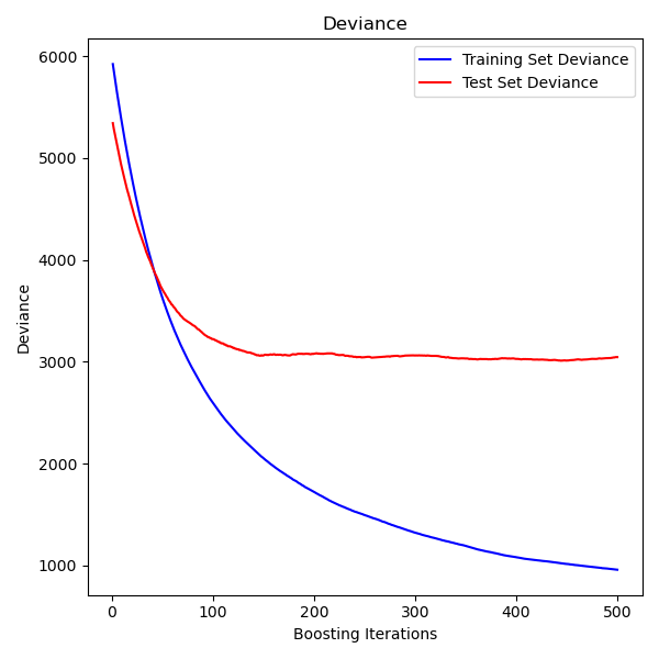
Plot training deviance

Finally, we will visualize the results. To do that we will first compute the test set deviance and then plot it against boosting iterations.

test_score = np.zeros((params["n_estimators"],), dtype=np.float64)
for i, y_pred in enumerate(reg.staged_predict(X_test)):
    test_score[i] = mean_squared_error(y_test, y_pred)

fig = plt.figure(figsize=(6, 6))
plt.subplot(1, 1, 1)
plt.title("Deviance")
plt.plot(
    np.arange(params["n_estimators"]) + 1,
    reg.train_score_,
    "b-",
    label="Training Set Deviance",
)
plt.plot(
    np.arange(params["n_estimators"]) + 1, test_score, "r-", label="Test Set Deviance"
)
plt.legend(loc="upper right")
plt.xlabel("Boosting Iterations")
plt.ylabel("Deviance")
fig.tight_layout()
plt.show()

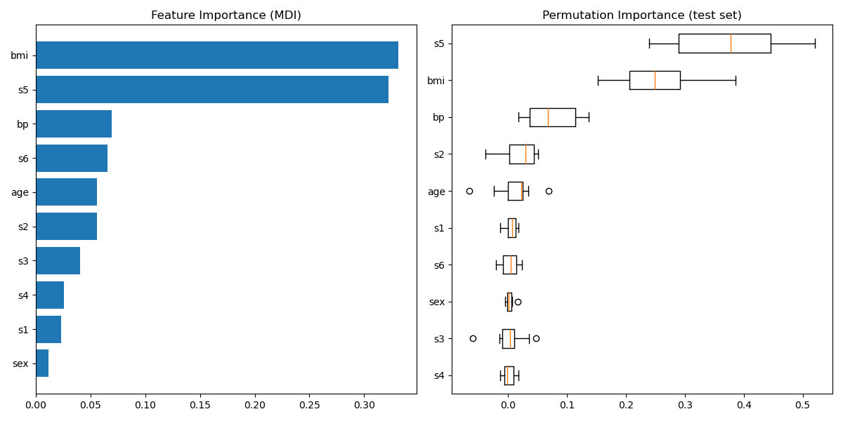
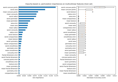
Plot feature importance

Warning

Careful, impurity-based feature importances can be misleading for high cardinality features (many unique values). As an alternative, the permutation importances of reg can be computed on a held out test set. See Permutation feature importance for more details.

For this example, the impurity-based and permutation methods identify the same 2 strongly predictive features but not in the same order. The third most predictive feature, “bp”, is also the same for the 2 methods. The remaining features are less predictive and the error bars of the permutation plot show that they overlap with 0.

feature_importance = reg.feature_importances_
sorted_idx = np.argsort(feature_importance)
pos = np.arange(sorted_idx.shape[0]) + 0.5
fig = plt.figure(figsize=(12, 6))
plt.subplot(1, 2, 1)
plt.barh(pos, feature_importance[sorted_idx], align="center")
plt.yticks(pos, np.array(diabetes.feature_names)[sorted_idx])
plt.title("Feature Importance (MDI)")

result = permutation_importance(
    reg, X_test, y_test, n_repeats=10, random_state=42, n_jobs=2
)
sorted_idx = result.importances_mean.argsort()
plt.subplot(1, 2, 2)
plt.boxplot(
    result.importances[sorted_idx].T,
    vert=False,
    labels=np.array(diabetes.feature_names)[sorted_idx],
)
plt.title("Permutation Importance (test set)")
fig.tight_layout()
plt.show()

Related examples

Gradient Boosting regularization

Gradient Boosting regularization

Feature importances with a forest of trees

Feature importances with a forest of trees

Gradient Boosting Out-of-Bag estimates

Gradient Boosting Out-of-Bag estimates

Permutation Importance vs Random Forest Feature Importance (MDI)

Permutation Importance vs Random Forest Feature Importance (MDI)