1.6. Nearest Neighbors#
sklearn.neighbors provides functionality for unsupervised and
supervised neighbors-based learning methods. Unsupervised nearest neighbors
is the foundation of many other learning methods,
notably manifold learning and spectral clustering. Supervised neighbors-based
learning comes in two flavors: classification for data with
discrete labels, and regression for data with continuous labels.
The principle behind nearest neighbor methods is to find a predefined number of training samples closest in distance to the new point, and predict the label from these. The number of samples can be a user-defined constant (k-nearest neighbor learning), or vary based on the local density of points (radius-based neighbor learning). The distance can, in general, be any metric measure: standard Euclidean distance is the most common choice. Neighbors-based methods are known as non-generalizing machine learning methods, since they simply “remember” all of its training data (possibly transformed into a fast indexing structure such as a Ball Tree or KD Tree).
Despite its simplicity, nearest neighbors has been successful in a large number of classification and regression problems, including handwritten digits and satellite image scenes. Being a non-parametric method, it is often successful in classification situations where the decision boundary is very irregular.
The classes in sklearn.neighbors can handle either NumPy arrays or
scipy.sparse matrices as input. For dense matrices, a large number of
possible distance metrics are supported. For sparse matrices, arbitrary
Minkowski metrics are supported for searches.
There are many learning routines which rely on nearest neighbors at their core. One example is kernel density estimation, discussed in the density estimation section.
1.6.1. Unsupervised Nearest Neighbors#
NearestNeighbors implements unsupervised nearest neighbors learning.
It acts as a uniform interface to three different nearest neighbors
algorithms: BallTree, KDTree, and a
brute-force algorithm based on routines in sklearn.metrics.pairwise.
The choice of neighbors search algorithm is controlled through the keyword
'algorithm', which must be one of
['auto', 'ball_tree', 'kd_tree', 'brute']. When the default value
'auto' is passed, the algorithm attempts to determine the best approach
from the training data. For a discussion of the strengths and weaknesses
of each option, see Nearest Neighbor Algorithms.
Warning
Regarding the Nearest Neighbors algorithms, if two neighbors \(k+1\) and \(k\) have identical distances but different labels, the result will depend on the ordering of the training data.
1.6.1.1. Finding the Nearest Neighbors#
For the simple task of finding the nearest neighbors between two sets of
data, the unsupervised algorithms within sklearn.neighbors can be
used:
>>> from sklearn.neighbors import NearestNeighbors
>>> import numpy as np
>>> X = np.array([[-1, -1], [-2, -1], [-3, -2], [1, 1], [2, 1], [3, 2]])
>>> nbrs = NearestNeighbors(n_neighbors=2, algorithm='ball_tree').fit(X)
>>> distances, indices = nbrs.kneighbors(X)
>>> indices
array([[0, 1],
       [1, 0],
       [2, 1],
       [3, 4],
       [4, 3],
       [5, 4]]...)
>>> distances
array([[0.        , 1.        ],
       [0.        , 1.        ],
       [0.        , 1.41421356],
       [0.        , 1.        ],
       [0.        , 1.        ],
       [0.        , 1.41421356]])
Because the query set matches the training set, the nearest neighbor of each point is the point itself, at a distance of zero.
It is also possible to efficiently produce a sparse graph showing the connections between neighboring points:
>>> nbrs.kneighbors_graph(X).toarray()
array([[1., 1., 0., 0., 0., 0.],
       [1., 1., 0., 0., 0., 0.],
       [0., 1., 1., 0., 0., 0.],
       [0., 0., 0., 1., 1., 0.],
       [0., 0., 0., 1., 1., 0.],
       [0., 0., 0., 0., 1., 1.]])
The dataset is structured such that points nearby in index order are nearby
in parameter space, leading to an approximately block-diagonal matrix of
K-nearest neighbors. Such a sparse graph is useful in a variety of
circumstances which make use of spatial relationships between points for
unsupervised learning: in particular, see Isomap,
LocallyLinearEmbedding, and
SpectralClustering.
1.6.1.2. KDTree and BallTree Classes#
Alternatively, one can use the KDTree or BallTree classes
directly to find nearest neighbors. This is the functionality wrapped by
the NearestNeighbors class used above. The Ball Tree and KD Tree
have the same interface; we’ll show an example of using the KD Tree here:
>>> from sklearn.neighbors import KDTree
>>> import numpy as np
>>> X = np.array([[-1, -1], [-2, -1], [-3, -2], [1, 1], [2, 1], [3, 2]])
>>> kdt = KDTree(X, leaf_size=30, metric='euclidean')
>>> kdt.query(X, k=2, return_distance=False)
array([[0, 1],
       [1, 0],
       [2, 1],
       [3, 4],
       [4, 3],
       [5, 4]]...)
Refer to the KDTree and BallTree class documentation
for more information on the options available for nearest neighbors searches,
including specification of query strategies, distance metrics, etc. For a list
of valid metrics use KDTree.valid_metrics and BallTree.valid_metrics:
>>> from sklearn.neighbors import KDTree, BallTree
>>> KDTree.valid_metrics
['euclidean', 'l2', 'minkowski', 'p', 'manhattan', 'cityblock', 'l1', 'chebyshev', 'infinity']
>>> BallTree.valid_metrics
['euclidean', 'l2', 'minkowski', 'p', 'manhattan', 'cityblock', 'l1', 'chebyshev', 'infinity', 'seuclidean', 'mahalanobis', 'hamming', 'canberra', 'braycurtis', 'jaccard', 'dice', 'rogerstanimoto', 'russellrao', 'sokalmichener', 'sokalsneath', 'haversine', 'pyfunc']
1.6.2. Nearest Neighbors Classification#
Neighbors-based classification is a type of instance-based learning or non-generalizing learning: it does not attempt to construct a general internal model, but simply stores instances of the training data. Classification is computed from a simple majority vote of the nearest neighbors of each point: a query point is assigned the data class which has the most representatives within the nearest neighbors of the point.
scikit-learn implements two different nearest neighbors classifiers:
KNeighborsClassifier implements learning based on the \(k\)
nearest neighbors of each query point, where \(k\) is an integer value
specified by the user. RadiusNeighborsClassifier implements learning
based on the number of neighbors within a fixed radius \(r\) of each
training point, where \(r\) is a floating-point value specified by
the user.
The \(k\)-neighbors classification in KNeighborsClassifier
is the most commonly used technique. The optimal choice of the value \(k\)
is highly data-dependent: in general a larger \(k\) suppresses the effects
of noise, but makes the classification boundaries less distinct.
In cases where the data is not uniformly sampled, radius-based neighbors
classification in RadiusNeighborsClassifier can be a better choice.
The user specifies a fixed radius \(r\), such that points in sparser
neighborhoods use fewer nearest neighbors for the classification. For
high-dimensional parameter spaces, this method becomes less effective due
to the so-called “curse of dimensionality”.
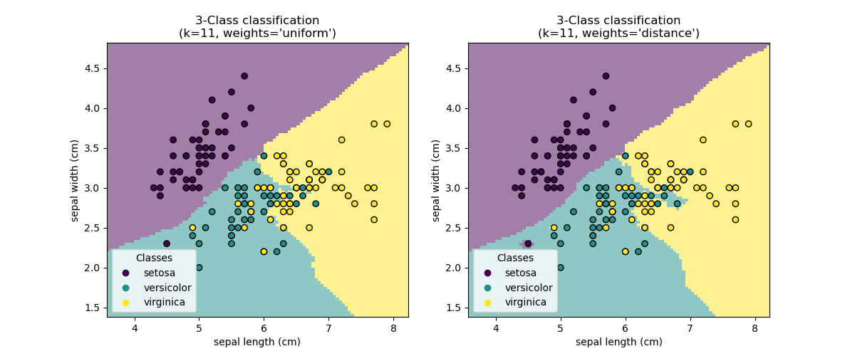
The basic nearest neighbors classification uses uniform weights: that is, the
value assigned to a query point is computed from a simple majority vote of
the nearest neighbors. Under some circumstances, it is better to weight the
neighbors such that nearer neighbors contribute more to the fit. This can
be accomplished through the weights keyword. The default value,
weights = 'uniform', assigns uniform weights to each neighbor.
weights = 'distance' assigns weights proportional to the inverse of the
distance from the query point. Alternatively, a user-defined function of the
distance can be supplied to compute the weights.
Examples
Nearest Neighbors Classification: an example of classification using nearest neighbors.
1.6.3. Nearest Neighbors Regression#
Neighbors-based regression can be used in cases where the data labels are continuous rather than discrete variables. The label assigned to a query point is computed based on the mean of the labels of its nearest neighbors.
scikit-learn implements two different neighbors regressors:
KNeighborsRegressor implements learning based on the \(k\)
nearest neighbors of each query point, where \(k\) is an integer
value specified by the user. RadiusNeighborsRegressor implements
learning based on the neighbors within a fixed radius \(r\) of the
query point, where \(r\) is a floating-point value specified by the
user.
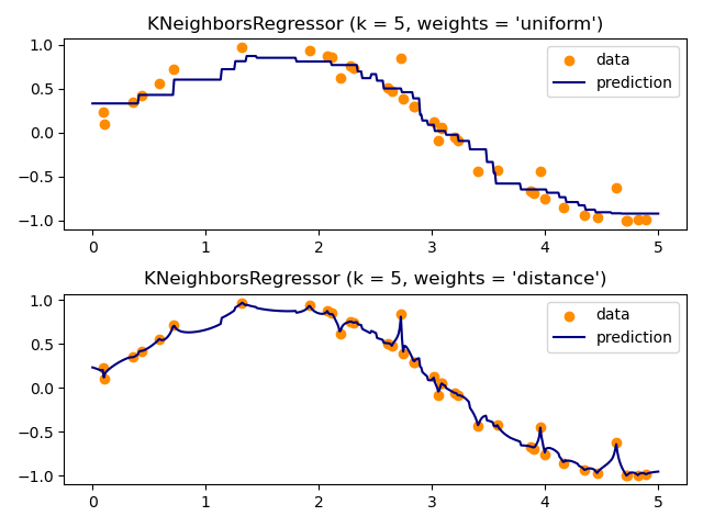
The basic nearest neighbors regression uses uniform weights: that is,
each point in the local neighborhood contributes uniformly to the
classification of a query point. Under some circumstances, it can be
advantageous to weight points such that nearby points contribute more
to the regression than faraway points. This can be accomplished through
the weights keyword. The default value, weights = 'uniform',
assigns equal weights to all points. weights = 'distance' assigns
weights proportional to the inverse of the distance from the query point.
Alternatively, a user-defined function of the distance can be supplied,
which will be used to compute the weights.
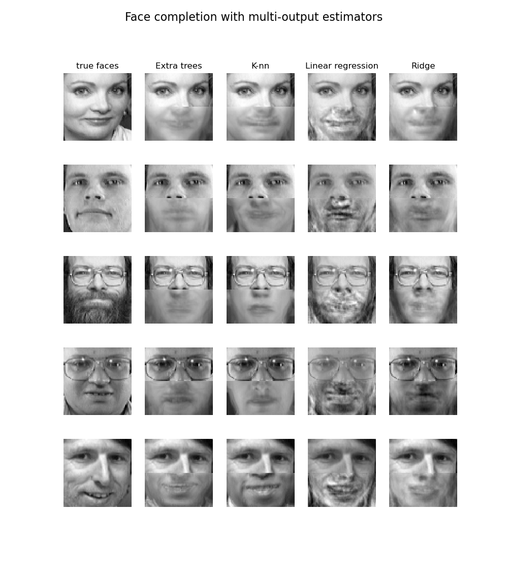
The use of multi-output nearest neighbors for regression is demonstrated in Face completion with a multi-output estimators. In this example, the inputs X are the pixels of the upper half of faces and the outputs Y are the pixels of the lower half of those faces.
Examples
Nearest Neighbors regression: an example of regression using nearest neighbors.
Face completion with a multi-output estimators: an example of multi-output regression using nearest neighbors.
1.6.4. Nearest Neighbor Algorithms#
1.6.4.1. Brute Force#
Fast computation of nearest neighbors is an active area of research in
machine learning. The most naive neighbor search implementation involves
the brute-force computation of distances between all pairs of points in the
dataset: for \(N\) samples in \(D\) dimensions, this approach scales
as \(O[D N^2]\). Efficient brute-force neighbors searches can be very
competitive for small data samples.
However, as the number of samples \(N\) grows, the brute-force
approach quickly becomes infeasible. In the classes within
sklearn.neighbors, brute-force neighbors searches are specified
using the keyword algorithm = 'brute', and are computed using the
routines available in sklearn.metrics.pairwise.
1.6.4.2. K-D Tree#
To address the computational inefficiencies of the brute-force approach, a variety of tree-based data structures have been invented. In general, these structures attempt to reduce the required number of distance calculations by efficiently encoding aggregate distance information for the sample. The basic idea is that if point \(A\) is very distant from point \(B\), and point \(B\) is very close to point \(C\), then we know that points \(A\) and \(C\) are very distant, without having to explicitly calculate their distance. In this way, the computational cost of a nearest neighbors search can be reduced to \(O[D N \log(N)]\) or better. This is a significant improvement over brute-force for large \(N\).
An early approach to taking advantage of this aggregate information was
the KD tree data structure (short for K-dimensional tree), which
generalizes two-dimensional Quad-trees and 3-dimensional Oct-trees
to an arbitrary number of dimensions. The KD tree is a binary tree
structure which recursively partitions the parameter space along the data
axes, dividing it into nested orthotropic regions into which data points
are filed. The construction of a KD tree is very fast: because partitioning
is performed only along the data axes, no \(D\)-dimensional distances
need to be computed. Once constructed, the nearest neighbor of a query
point can be determined with only \(O[\log(N)]\) distance computations.
Though the KD tree approach is very fast for low-dimensional (\(D < 20\))
neighbors searches, it becomes inefficient as \(D\) grows very large:
this is one manifestation of the so-called “curse of dimensionality”.
In scikit-learn, KD tree neighbors searches are specified using the
keyword algorithm = 'kd_tree', and are computed using the class
KDTree.
References#
“Multidimensional binary search trees used for associative searching”, Bentley, J.L., Communications of the ACM (1975)
1.6.4.3. Ball Tree#
To address the inefficiencies of KD Trees in higher dimensions, the ball tree data structure was developed. Where KD trees partition data along Cartesian axes, ball trees partition data in a series of nesting hyper-spheres. This makes tree construction more costly than that of the KD tree, but results in a data structure which can be very efficient on highly structured data, even in very high dimensions.
A ball tree recursively divides the data into nodes defined by a centroid \(C\) and radius \(r\), such that each point in the node lies within the hyper-sphere defined by \(r\) and \(C\). The number of candidate points for a neighbor search is reduced through use of the triangle inequality:
With this setup, a single distance calculation between a test point and
the centroid is sufficient to determine a lower and upper bound on the
distance to all points within the node.
Because of the spherical geometry of the ball tree nodes, it can out-perform
a KD-tree in high dimensions, though the actual performance is highly
dependent on the structure of the training data.
In scikit-learn, ball-tree-based
neighbors searches are specified using the keyword algorithm = 'ball_tree',
and are computed using the class BallTree.
Alternatively, the user can work with the BallTree class directly.
References#
“Five Balltree Construction Algorithms”, Omohundro, S.M., International Computer Science Institute Technical Report (1989)
Choice of Nearest Neighbors Algorithm#
The optimal algorithm for a given dataset is a complicated choice, and depends on a number of factors:
number of samples \(N\) (i.e.
n_samples) and dimensionality \(D\) (i.e.n_features).Brute force query time grows as \(O[D N]\)
Ball tree query time grows as approximately \(O[D \log(N)]\)
KD tree query time changes with \(D\) in a way that is difficult to precisely characterise. For small \(D\) (less than 20 or so) the cost is approximately \(O[D\log(N)]\), and the KD tree query can be very efficient. For larger \(D\), the cost increases to nearly \(O[DN]\), and the overhead due to the tree structure can lead to queries which are slower than brute force.
For small data sets (\(N\) less than 30 or so), \(\log(N)\) is comparable to \(N\), and brute force algorithms can be more efficient than a tree-based approach. Both
KDTreeandBallTreeaddress this through providing a leaf size parameter: this controls the number of samples at which a query switches to brute-force. This allows both algorithms to approach the efficiency of a brute-force computation for small \(N\).data structure: intrinsic dimensionality of the data and/or sparsity of the data. Intrinsic dimensionality refers to the dimension \(d \le D\) of a manifold on which the data lies, which can be linearly or non-linearly embedded in the parameter space. Sparsity refers to the degree to which the data fills the parameter space (this is to be distinguished from the concept as used in “sparse” matrices. The data matrix may have no zero entries, but the structure can still be “sparse” in this sense).
Brute force query time is unchanged by data structure.
Ball tree and KD tree query times can be greatly influenced by data structure. In general, sparser data with a smaller intrinsic dimensionality leads to faster query times. Because the KD tree internal representation is aligned with the parameter axes, it will not generally show as much improvement as ball tree for arbitrarily structured data.
Datasets used in machine learning tend to be very structured, and are very well-suited for tree-based queries.
number of neighbors \(k\) requested for a query point.
Brute force query time is largely unaffected by the value of \(k\)
Ball tree and KD tree query time will become slower as \(k\) increases. This is due to two effects: first, a larger \(k\) leads to the necessity to search a larger portion of the parameter space. Second, using \(k > 1\) requires internal queueing of results as the tree is traversed.
As \(k\) becomes large compared to \(N\), the ability to prune branches in a tree-based query is reduced. In this situation, Brute force queries can be more efficient.
number of query points. Both the ball tree and the KD Tree require a construction phase. The cost of this construction becomes negligible when amortized over many queries. If only a small number of queries will be performed, however, the construction can make up a significant fraction of the total cost. If very few query points will be required, brute force is better than a tree-based method.
Currently, algorithm = 'auto' selects 'brute' if any of the following
conditions are verified:
input data is sparse
metric = 'precomputed'\(D > 15\)
\(k >= N/2\)
effective_metric_isn’t in theVALID_METRICSlist for either'kd_tree'or'ball_tree'
Otherwise, it selects the first out of 'kd_tree' and 'ball_tree' that
has effective_metric_ in its VALID_METRICS list. This heuristic is
based on the following assumptions:
the number of query points is at least the same order as the number of training points
leaf_sizeis close to its default value of30when \(D > 15\), the intrinsic dimensionality of the data is generally too high for tree-based methods
Effect of leaf_size#
As noted above, for small sample sizes a brute force search can be more
efficient than a tree-based query. This fact is accounted for in the ball
tree and KD tree by internally switching to brute force searches within
leaf nodes. The level of this switch can be specified with the parameter
leaf_size. This parameter choice has many effects:
- construction time
A larger
leaf_sizeleads to a faster tree construction time, because fewer nodes need to be created- query time
Both a large or small
leaf_sizecan lead to suboptimal query cost. Forleaf_sizeapproaching 1, the overhead involved in traversing nodes can significantly slow query times. Forleaf_sizeapproaching the size of the training set, queries become essentially brute force. A good compromise between these isleaf_size = 30, the default value of the parameter.- memory
As
leaf_sizeincreases, the memory required to store a tree structure decreases. This is especially important in the case of ball tree, which stores a \(D\)-dimensional centroid for each node. The required storage space forBallTreeis approximately1 / leaf_sizetimes the size of the training set.
leaf_size is not referenced for brute force queries.
Valid Metrics for Nearest Neighbor Algorithms#
For a list of available metrics, see the documentation of the
DistanceMetric class and the metrics listed in
sklearn.metrics.pairwise.PAIRWISE_DISTANCE_FUNCTIONS. Note that the “cosine”
metric uses cosine_distances.
A list of valid metrics for any of the above algorithms can be obtained by using their
valid_metric attribute. For example, valid metrics for KDTree can be generated by:
>>> from sklearn.neighbors import KDTree
>>> print(sorted(KDTree.valid_metrics))
['chebyshev', 'cityblock', 'euclidean', 'infinity', 'l1', 'l2', 'manhattan', 'minkowski', 'p']
1.6.5. Nearest Centroid Classifier#
The NearestCentroid classifier is a simple algorithm that represents
each class by the centroid of its members. In effect, this makes it
similar to the label updating phase of the KMeans algorithm.
It also has no parameters to choose, making it a good baseline classifier. It
does, however, suffer on non-convex classes, as well as when classes have
drastically different variances, as equal variance in all dimensions is
assumed. See Linear Discriminant Analysis (LinearDiscriminantAnalysis)
and Quadratic Discriminant Analysis (QuadraticDiscriminantAnalysis)
for more complex methods that do not make this assumption. Usage of the default
NearestCentroid is simple:
>>> from sklearn.neighbors import NearestCentroid
>>> import numpy as np
>>> X = np.array([[-1, -1], [-2, -1], [-3, -2], [1, 1], [2, 1], [3, 2]])
>>> y = np.array([1, 1, 1, 2, 2, 2])
>>> clf = NearestCentroid()
>>> clf.fit(X, y)
NearestCentroid()
>>> print(clf.predict([[-0.8, -1]]))
[1]
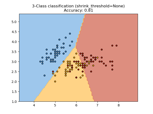
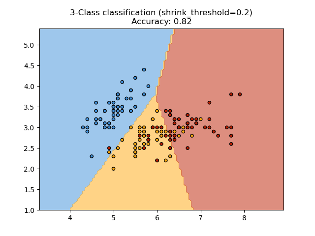
1.6.5.1. Nearest Shrunken Centroid#
The NearestCentroid classifier has a shrink_threshold parameter,
which implements the nearest shrunken centroid classifier. In effect, the value
of each feature for each centroid is divided by the within-class variance of
that feature. The feature values are then reduced by shrink_threshold. Most
notably, if a particular feature value crosses zero, it is set
to zero. In effect, this removes the feature from affecting the classification.
This is useful, for example, for removing noisy features.
In the example below, using a small shrink threshold increases the accuracy of the model from 0.81 to 0.82.
Examples
Nearest Centroid Classification: an example of classification using nearest centroid with different shrink thresholds.
1.6.6. Nearest Neighbors Transformer#
Many scikit-learn estimators rely on nearest neighbors: Several classifiers and
regressors such as KNeighborsClassifier and
KNeighborsRegressor, but also some clustering methods such as
DBSCAN and
SpectralClustering, and some manifold embeddings such
as TSNE and Isomap.
All these estimators can compute internally the nearest neighbors, but most of
them also accept precomputed nearest neighbors sparse graph,
as given by kneighbors_graph and
radius_neighbors_graph. With mode
mode='connectivity', these functions return a binary adjacency sparse graph
as required, for instance, in SpectralClustering.
Whereas with mode='distance', they return a distance sparse graph as required,
for instance, in DBSCAN. To include these functions in
a scikit-learn pipeline, one can also use the corresponding classes
KNeighborsTransformer and RadiusNeighborsTransformer.
The benefits of this sparse graph API are multiple.
First, the precomputed graph can be reused multiple times, for instance while varying a parameter of the estimator. This can be done manually by the user, or using the caching properties of the scikit-learn pipeline:
>>> import tempfile
>>> from sklearn.manifold import Isomap
>>> from sklearn.neighbors import KNeighborsTransformer
>>> from sklearn.pipeline import make_pipeline
>>> from sklearn.datasets import make_regression
>>> cache_path = tempfile.gettempdir()  # we use a temporary folder here
>>> X, _ = make_regression(n_samples=50, n_features=25, random_state=0)
>>> estimator = make_pipeline(
...     KNeighborsTransformer(mode='distance'),
...     Isomap(n_components=3, metric='precomputed'),
...     memory=cache_path)
>>> X_embedded = estimator.fit_transform(X)
>>> X_embedded.shape
(50, 3)
Second, precomputing the graph can give finer control on the nearest neighbors
estimation, for instance enabling multiprocessing though the parameter
n_jobs, which might not be available in all estimators.
Finally, the precomputation can be performed by custom estimators to use
different implementations, such as approximate nearest neighbors methods, or
implementation with special data types. The precomputed neighbors
sparse graph needs to be formatted as in
radius_neighbors_graph output:
a CSR matrix (although COO, CSC or LIL will be accepted).
only explicitly store nearest neighborhoods of each sample with respect to the training data. This should include those at 0 distance from a query point, including the matrix diagonal when computing the nearest neighborhoods between the training data and itself.
each row’s
datashould store the distance in increasing order (optional. Unsorted data will be stable-sorted, adding a computational overhead).all values in data should be non-negative.
there should be no duplicate
indicesin any row (see scipy/scipy#5807).if the algorithm being passed the precomputed matrix uses k nearest neighbors (as opposed to radius neighborhood), at least k neighbors must be stored in each row (or k+1, as explained in the following note).
Note
When a specific number of neighbors is queried (using
KNeighborsTransformer), the definition of n_neighbors is ambiguous
since it can either include each training point as its own neighbor, or
exclude them. Neither choice is perfect, since including them leads to a
different number of non-self neighbors during training and testing, while
excluding them leads to a difference between fit(X).transform(X) and
fit_transform(X), which is against scikit-learn API.
In KNeighborsTransformer we use the definition which includes each
training point as its own neighbor in the count of n_neighbors. However,
for compatibility reasons with other estimators which use the other
definition, one extra neighbor will be computed when mode == 'distance'.
To maximise compatibility with all estimators, a safe choice is to always
include one extra neighbor in a custom nearest neighbors estimator, since
unnecessary neighbors will be filtered by following estimators.
Examples
Approximate nearest neighbors in TSNE: an example of pipelining
KNeighborsTransformerandTSNE. Also proposes two custom nearest neighbors estimators based on external packages.Caching nearest neighbors: an example of pipelining
KNeighborsTransformerandKNeighborsClassifierto enable caching of the neighbors graph during a hyper-parameter grid-search.
1.6.7. Neighborhood Components Analysis#
Neighborhood Components Analysis (NCA, NeighborhoodComponentsAnalysis)
is a distance metric learning algorithm which aims to improve the accuracy of
nearest neighbors classification compared to the standard Euclidean distance.
The algorithm directly maximizes a stochastic variant of the leave-one-out
k-nearest neighbors (KNN) score on the training set. It can also learn a
low-dimensional linear projection of data that can be used for data
visualization and fast classification.
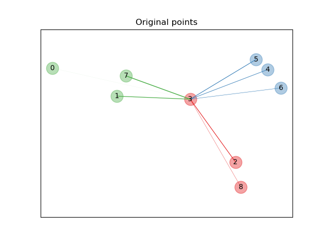
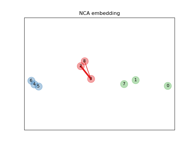
In the above illustrating figure, we consider some points from a randomly generated dataset. We focus on the stochastic KNN classification of point no. 3. The thickness of a link between sample 3 and another point is proportional to their distance, and can be seen as the relative weight (or probability) that a stochastic nearest neighbor prediction rule would assign to this point. In the original space, sample 3 has many stochastic neighbors from various classes, so the right class is not very likely. However, in the projected space learned by NCA, the only stochastic neighbors with non-negligible weight are from the same class as sample 3, guaranteeing that the latter will be well classified. See the mathematical formulation for more details.
1.6.7.1. Classification#
Combined with a nearest neighbors classifier (KNeighborsClassifier),
NCA is attractive for classification because it can naturally handle
multi-class problems without any increase in the model size, and does not
introduce additional parameters that require fine-tuning by the user.
NCA classification has been shown to work well in practice for data sets of varying size and difficulty. In contrast to related methods such as Linear Discriminant Analysis, NCA does not make any assumptions about the class distributions. The nearest neighbor classification can naturally produce highly irregular decision boundaries.
To use this model for classification, one needs to combine a
NeighborhoodComponentsAnalysis instance that learns the optimal
transformation with a KNeighborsClassifier instance that performs the
classification in the projected space. Here is an example using the two
classes:
>>> from sklearn.neighbors import (NeighborhoodComponentsAnalysis,
... KNeighborsClassifier)
>>> from sklearn.datasets import load_iris
>>> from sklearn.model_selection import train_test_split
>>> from sklearn.pipeline import Pipeline
>>> X, y = load_iris(return_X_y=True)
>>> X_train, X_test, y_train, y_test = train_test_split(X, y,
... stratify=y, test_size=0.7, random_state=42)
>>> nca = NeighborhoodComponentsAnalysis(random_state=42)
>>> knn = KNeighborsClassifier(n_neighbors=3)
>>> nca_pipe = Pipeline([('nca', nca), ('knn', knn)])
>>> nca_pipe.fit(X_train, y_train)
Pipeline(...)
>>> print(nca_pipe.score(X_test, y_test))
0.96190476...
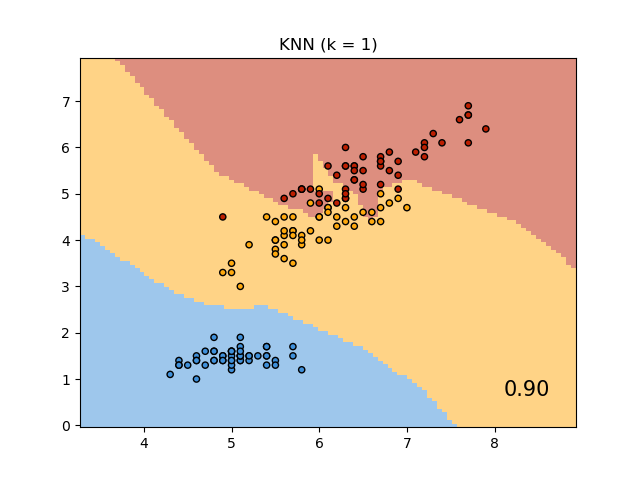
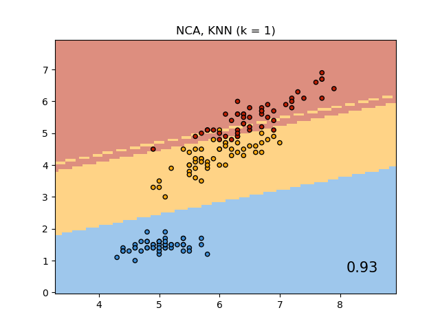
The plot shows decision boundaries for Nearest Neighbor Classification and Neighborhood Components Analysis classification on the iris dataset, when training and scoring on only two features, for visualisation purposes.
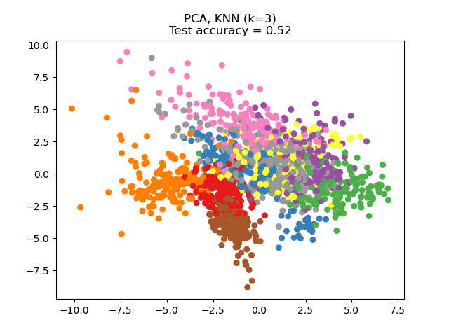
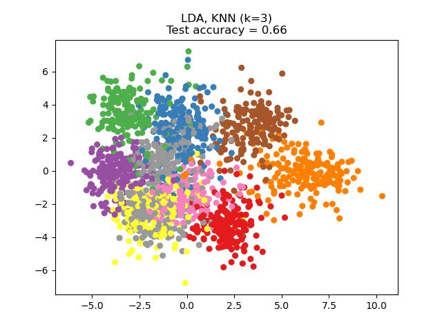
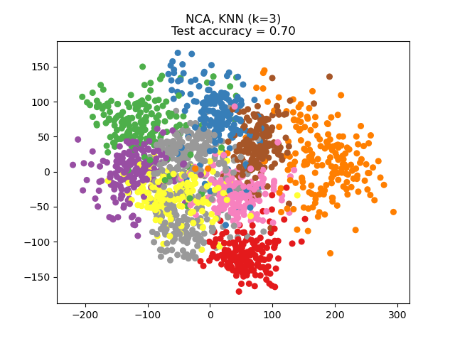
1.6.7.2. Dimensionality reduction#
NCA can be used to perform supervised dimensionality reduction. The input data
are projected onto a linear subspace consisting of the directions which
minimize the NCA objective. The desired dimensionality can be set using the
parameter n_components. For instance, the following figure shows a
comparison of dimensionality reduction with Principal Component Analysis
(PCA), Linear Discriminant Analysis
(LinearDiscriminantAnalysis) and
Neighborhood Component Analysis (NeighborhoodComponentsAnalysis) on
the Digits dataset, a dataset with size \(n_{samples} = 1797\) and
\(n_{features} = 64\). The data set is split into a training and a test set
of equal size, then standardized. For evaluation the 3-nearest neighbor
classification accuracy is computed on the 2-dimensional projected points found
by each method. Each data sample belongs to one of 10 classes.
Examples
1.6.7.3. Mathematical formulation#
The goal of NCA is to learn an optimal linear transformation matrix of size
(n_components, n_features), which maximises the sum over all samples
\(i\) of the probability \(p_i\) that \(i\) is correctly
classified, i.e.:
with \(N\) = n_samples and \(p_i\) the probability of sample
\(i\) being correctly classified according to a stochastic nearest
neighbors rule in the learned embedded space:
where \(C_i\) is the set of points in the same class as sample \(i\), and \(p_{i j}\) is the softmax over Euclidean distances in the embedded space:
Mahalanobis distance#
NCA can be seen as learning a (squared) Mahalanobis distance metric:
where \(M = L^T L\) is a symmetric positive semi-definite matrix of size
(n_features, n_features).
1.6.7.4. Implementation#
This implementation follows what is explained in the original paper [1]. For the optimisation method, it currently uses scipy’s L-BFGS-B with a full gradient computation at each iteration, to avoid to tune the learning rate and provide stable learning.
See the examples below and the docstring of
NeighborhoodComponentsAnalysis.fit for further information.
1.6.7.5. Complexity#
1.6.7.5.1. Training#
NCA stores a matrix of pairwise distances, taking n_samples ** 2 memory.
Time complexity depends on the number of iterations done by the optimisation
algorithm. However, one can set the maximum number of iterations with the
argument max_iter. For each iteration, time complexity is
O(n_components x n_samples x min(n_samples, n_features)).
1.6.7.5.2. Transform#
Here the transform operation returns \(LX^T\), therefore its time
complexity equals n_components * n_features * n_samples_test. There is no
added space complexity in the operation.
References