3.2. Tuning the hyper-parameters of an estimator#
Hyper-parameters are parameters that are not directly learnt within estimators.
In scikit-learn they are passed as arguments to the constructor of the
estimator classes. Typical examples include C, kernel and gamma
for Support Vector Classifier, alpha for Lasso, etc.
It is possible and recommended to search the hyper-parameter space for the best cross validation score.
Any parameter provided when constructing an estimator may be optimized in this manner. Specifically, to find the names and current values for all parameters for a given estimator, use:
estimator.get_params()
A search consists of:
an estimator (regressor or classifier such as
sklearn.svm.SVC());a parameter space;
a method for searching or sampling candidates;
a cross-validation scheme; and
Two generic approaches to parameter search are provided in
scikit-learn: for given values, GridSearchCV exhaustively considers
all parameter combinations, while RandomizedSearchCV can sample a
given number of candidates from a parameter space with a specified
distribution. Both these tools have successive halving counterparts
HalvingGridSearchCV and HalvingRandomSearchCV, which can be
much faster at finding a good parameter combination.
After describing these tools we detail best practices applicable to these approaches. Some models allow for specialized, efficient parameter search strategies, outlined in Alternatives to brute force parameter search.
Note that it is common that a small subset of those parameters can have a large impact on the predictive or computation performance of the model while others can be left to their default values. It is recommended to read the docstring of the estimator class to get a finer understanding of their expected behavior, possibly by reading the enclosed reference to the literature.
3.2.1. Exhaustive Grid Search#
The grid search provided by GridSearchCV exhaustively generates
candidates from a grid of parameter values specified with the param_grid
parameter. For instance, the following param_grid:
param_grid = [
  {'C': [1, 10, 100, 1000], 'kernel': ['linear']},
  {'C': [1, 10, 100, 1000], 'gamma': [0.001, 0.0001], 'kernel': ['rbf']},
 ]
specifies that two grids should be explored: one with a linear kernel and C values in [1, 10, 100, 1000], and the second one with an RBF kernel, and the cross-product of C values ranging in [1, 10, 100, 1000] and gamma values in [0.001, 0.0001].
The GridSearchCV instance implements the usual estimator API: when
“fitting” it on a dataset all the possible combinations of parameter values are
evaluated and the best combination is retained.
Examples
See Nested versus non-nested cross-validation for an example of Grid Search within a cross validation loop on the iris dataset. This is the best practice for evaluating the performance of a model with grid search.
See Sample pipeline for text feature extraction and evaluation for an example of Grid Search coupling parameters from a text documents feature extractor (n-gram count vectorizer and TF-IDF transformer) with a classifier (here a linear SVM trained with SGD with either elastic net or L2 penalty) using a
Pipelineinstance.
Advanced examples#
See Nested versus non-nested cross-validation for an example of Grid Search within a cross validation loop on the iris dataset. This is the best practice for evaluating the performance of a model with grid search.
See Demonstration of multi-metric evaluation on cross_val_score and GridSearchCV for an example of
GridSearchCVbeing used to evaluate multiple metrics simultaneously.See Balance model complexity and cross-validated score for an example of using
refit=callableinterface inGridSearchCV. The example shows how this interface adds a certain amount of flexibility in identifying the “best” estimator. This interface can also be used in multiple metrics evaluation.See Statistical comparison of models using grid search for an example of how to do a statistical comparison on the outputs of
GridSearchCV.
3.2.2. Randomized Parameter Optimization#
While using a grid of parameter settings is currently the most widely used
method for parameter optimization, other search methods have more
favorable properties.
RandomizedSearchCV implements a randomized search over parameters,
where each setting is sampled from a distribution over possible parameter values.
This has two main benefits over an exhaustive search:
A budget can be chosen independent of the number of parameters and possible values.
Adding parameters that do not influence the performance does not decrease efficiency.
Specifying how parameters should be sampled is done using a dictionary, very
similar to specifying parameters for GridSearchCV. Additionally,
a computation budget, being the number of sampled candidates or sampling
iterations, is specified using the n_iter parameter.
For each parameter, either a distribution over possible values or a list of
discrete choices (which will be sampled uniformly) can be specified:
{'C': scipy.stats.expon(scale=100), 'gamma': scipy.stats.expon(scale=.1),
  'kernel': ['rbf'], 'class_weight':['balanced', None]}
This example uses the scipy.stats module, which contains many useful
distributions for sampling parameters, such as expon, gamma,
uniform, loguniform or randint.
In principle, any function can be passed that provides a rvs (random
variate sample) method to sample a value. A call to the rvs function should
provide independent random samples from possible parameter values on
consecutive calls.
Warning
The distributions in scipy.stats prior to version scipy 0.16
do not allow specifying a random state. Instead, they use the global
numpy random state, that can be seeded via np.random.seed or set
using np.random.set_state. However, beginning scikit-learn 0.18,
the sklearn.model_selection module sets the random state provided
by the user if scipy >= 0.16 is also available.
For continuous parameters, such as C above, it is important to specify
a continuous distribution to take full advantage of the randomization. This way,
increasing n_iter will always lead to a finer search.
A continuous log-uniform random variable is the continuous version of
a log-spaced parameter. For example to specify the equivalent of C from above,
loguniform(1, 100) can be used instead of [1, 10, 100].
Mirroring the example above in grid search, we can specify a continuous random
variable that is log-uniformly distributed between 1e0 and 1e3:
from sklearn.utils.fixes import loguniform
{'C': loguniform(1e0, 1e3),
 'gamma': loguniform(1e-4, 1e-3),
 'kernel': ['rbf'],
 'class_weight':['balanced', None]}
Examples
Comparing randomized search and grid search for hyperparameter estimation compares the usage and efficiency of randomized search and grid search.
References
Bergstra, J. and Bengio, Y., Random search for hyper-parameter optimization, The Journal of Machine Learning Research (2012)
3.2.3. Searching for optimal parameters with successive halving#
Scikit-learn also provides the HalvingGridSearchCV and
HalvingRandomSearchCV estimators that can be used to
search a parameter space using successive halving [1] [2]. Successive
halving (SH) is like a tournament among candidate parameter combinations.
SH is an iterative selection process where all candidates (the
parameter combinations) are evaluated with a small amount of resources at
the first iteration. Only some of these candidates are selected for the next
iteration, which will be allocated more resources. For parameter tuning, the
resource is typically the number of training samples, but it can also be an
arbitrary numeric parameter such as n_estimators in a random forest.
Note
The resource increase chosen should be large enough so that a large improvement in scores is obtained when taking into account statistical significance.
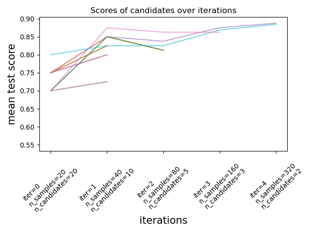
As illustrated in the figure below, only a subset of candidates ‘survive’ until the last iteration. These are the candidates that have consistently ranked among the top-scoring candidates across all iterations. Each iteration is allocated an increasing amount of resources per candidate, here the number of samples.
We here briefly describe the main parameters, but each parameter and their
interactions are described more in detail in the dropdown section below. The
factor (> 1) parameter controls the rate at which the resources grow, and
the rate at which the number of candidates decreases. In each iteration, the
number of resources per candidate is multiplied by factor and the number
of candidates is divided by the same factor. Along with resource and
min_resources, factor is the most important parameter to control the
search in our implementation, though a value of 3 usually works well.
factor effectively controls the number of iterations in
HalvingGridSearchCV and the number of candidates (by default) and
iterations in HalvingRandomSearchCV. aggressive_elimination=True
can also be used if the number of available resources is small. More control
is available through tuning the min_resources parameter.
These estimators are still experimental: their predictions
and their API might change without any deprecation cycle. To use them, you
need to explicitly import enable_halving_search_cv:
>>> from sklearn.experimental import enable_halving_search_cv  # noqa
>>> from sklearn.model_selection import HalvingGridSearchCV
>>> from sklearn.model_selection import HalvingRandomSearchCV
Examples
The sections below dive into technical aspects of successive halving.
Choosing min_resources and the number of candidates#
Beside factor, the two main parameters that influence the behaviour of a
successive halving search are the min_resources parameter, and the
number of candidates (or parameter combinations) that are evaluated.
min_resources is the amount of resources allocated at the first
iteration for each candidate. The number of candidates is specified directly
in HalvingRandomSearchCV, and is determined from the param_grid
parameter of HalvingGridSearchCV.
Consider a case where the resource is the number of samples, and where we
have 1000 samples. In theory, with min_resources=10 and factor=2, we
are able to run at most 7 iterations with the following number of
samples: [10, 20, 40, 80, 160, 320, 640].
But depending on the number of candidates, we might run less than 7
iterations: if we start with a small number of candidates, the last
iteration might use less than 640 samples, which means not using all the
available resources (samples). For example if we start with 5 candidates, we
only need 2 iterations: 5 candidates for the first iteration, then
5 // 2 = 2 candidates at the second iteration, after which we know which
candidate performs the best (so we don’t need a third one). We would only be
using at most 20 samples which is a waste since we have 1000 samples at our
disposal. On the other hand, if we start with a high number of
candidates, we might end up with a lot of candidates at the last iteration,
which may not always be ideal: it means that many candidates will run with
the full resources, basically reducing the procedure to standard search.
In the case of HalvingRandomSearchCV, the number of candidates is set
by default such that the last iteration uses as much of the available
resources as possible. For HalvingGridSearchCV, the number of
candidates is determined by the param_grid parameter. Changing the value of
min_resources will impact the number of possible iterations, and as a
result will also have an effect on the ideal number of candidates.
Another consideration when choosing min_resources is whether or not it
is easy to discriminate between good and bad candidates with a small amount
of resources. For example, if you need a lot of samples to distinguish
between good and bad parameters, a high min_resources is recommended. On
the other hand if the distinction is clear even with a small amount of
samples, then a small min_resources may be preferable since it would
speed up the computation.
Notice in the example above that the last iteration does not use the maximum
amount of resources available: 1000 samples are available, yet only 640 are
used, at most. By default, both HalvingRandomSearchCV and
HalvingGridSearchCV try to use as many resources as possible in the
last iteration, with the constraint that this amount of resources must be a
multiple of both min_resources and factor (this constraint will be clear
in the next section). HalvingRandomSearchCV achieves this by
sampling the right amount of candidates, while HalvingGridSearchCV
achieves this by properly setting min_resources.
Amount of resource and number of candidates at each iteration#
At any iteration i, each candidate is allocated a given amount of resources
which we denote n_resources_i. This quantity is controlled by the
parameters factor and min_resources as follows (factor is strictly
greater than 1):
n_resources_i = factor**i * min_resources,
or equivalently:
n_resources_{i+1} = n_resources_i * factor
where min_resources == n_resources_0 is the amount of resources used at
the first iteration. factor also defines the proportions of candidates
that will be selected for the next iteration:
n_candidates_i = n_candidates // (factor ** i)
or equivalently:
n_candidates_0 = n_candidates
n_candidates_{i+1} = n_candidates_i // factor
So in the first iteration, we use min_resources resources
n_candidates times. In the second iteration, we use min_resources *
factor resources n_candidates // factor times. The third again
multiplies the resources per candidate and divides the number of candidates.
This process stops when the maximum amount of resource per candidate is
reached, or when we have identified the best candidate. The best candidate
is identified at the iteration that is evaluating factor or less candidates
(see just below for an explanation).
Here is an example with min_resources=3 and factor=2, starting with
70 candidates:
|
|
|---|---|
3 (=min_resources) |
70 (=n_candidates) |
3 * 2 = 6 |
70 // 2 = 35 |
6 * 2 = 12 |
35 // 2 = 17 |
12 * 2 = 24 |
17 // 2 = 8 |
24 * 2 = 48 |
8 // 2 = 4 |
48 * 2 = 96 |
4 // 2 = 2 |
We can note that:
the process stops at the first iteration which evaluates
factor=2candidates: the best candidate is the best out of these 2 candidates. It is not necessary to run an additional iteration, since it would only evaluate one candidate (namely the best one, which we have already identified). For this reason, in general, we want the last iteration to run at mostfactorcandidates. If the last iteration evaluates more thanfactorcandidates, then this last iteration reduces to a regular search (as inRandomizedSearchCVorGridSearchCV).each
n_resources_iis a multiple of bothfactorandmin_resources(which is confirmed by its definition above).
The amount of resources that is used at each iteration can be found in the
n_resources_ attribute.
Choosing a resource#
By default, the resource is defined in terms of number of samples. That is,
each iteration will use an increasing amount of samples to train on. You can
however manually specify a parameter to use as the resource with the
resource parameter. Here is an example where the resource is defined in
terms of the number of estimators of a random forest:
>>> from sklearn.datasets import make_classification
>>> from sklearn.ensemble import RandomForestClassifier
>>> from sklearn.experimental import enable_halving_search_cv  # noqa
>>> from sklearn.model_selection import HalvingGridSearchCV
>>> import pandas as pd
>>> param_grid = {'max_depth': [3, 5, 10],
...               'min_samples_split': [2, 5, 10]}
>>> base_estimator = RandomForestClassifier(random_state=0)
>>> X, y = make_classification(n_samples=1000, random_state=0)
>>> sh = HalvingGridSearchCV(base_estimator, param_grid, cv=5,
...                          factor=2, resource='n_estimators',
...                          max_resources=30).fit(X, y)
>>> sh.best_estimator_
RandomForestClassifier(max_depth=5, n_estimators=24, random_state=0)
Note that it is not possible to budget on a parameter that is part of the parameter grid.
Exhausting the available resources#
As mentioned above, the number of resources that is used at each iteration
depends on the min_resources parameter.
If you have a lot of resources available but start with a low number of
resources, some of them might be wasted (i.e. not used):
>>> from sklearn.datasets import make_classification
>>> from sklearn.svm import SVC
>>> from sklearn.experimental import enable_halving_search_cv  # noqa
>>> from sklearn.model_selection import HalvingGridSearchCV
>>> import pandas as pd
>>> param_grid= {'kernel': ('linear', 'rbf'),
...              'C': [1, 10, 100]}
>>> base_estimator = SVC(gamma='scale')
>>> X, y = make_classification(n_samples=1000)
>>> sh = HalvingGridSearchCV(base_estimator, param_grid, cv=5,
...                          factor=2, min_resources=20).fit(X, y)
>>> sh.n_resources_
[20, 40, 80]
The search process will only use 80 resources at most, while our maximum
amount of available resources is n_samples=1000. Here, we have
min_resources = r_0 = 20.
For HalvingGridSearchCV, by default, the min_resources parameter
is set to ‘exhaust’. This means that min_resources is automatically set
such that the last iteration can use as many resources as possible, within
the max_resources limit:
>>> sh = HalvingGridSearchCV(base_estimator, param_grid, cv=5,
...                          factor=2, min_resources='exhaust').fit(X, y)
>>> sh.n_resources_
[250, 500, 1000]
min_resources was here automatically set to 250, which results in the last
iteration using all the resources. The exact value that is used depends on
the number of candidate parameters, on max_resources and on factor.
For HalvingRandomSearchCV, exhausting the resources can be done in 2
ways:
by setting
min_resources='exhaust', just like forHalvingGridSearchCV;by setting
n_candidates='exhaust'.
Both options are mutually exclusive: using min_resources='exhaust' requires
knowing the number of candidates, and symmetrically n_candidates='exhaust'
requires knowing min_resources.
In general, exhausting the total number of resources leads to a better final candidate parameter, and is slightly more time-intensive.
3.2.3.1. Aggressive elimination of candidates#
Using the aggressive_elimination parameter, you can force the search
process to end up with less than factor candidates at the last
iteration.
Code example of aggressive elimination#
Ideally, we want the last iteration to evaluate factor candidates. We
then just have to pick the best one. When the number of available resources is
small with respect to the number of candidates, the last iteration may have to
evaluate more than factor candidates:
>>> from sklearn.datasets import make_classification
>>> from sklearn.svm import SVC
>>> from sklearn.experimental import enable_halving_search_cv  # noqa
>>> from sklearn.model_selection import HalvingGridSearchCV
>>> import pandas as pd
>>> param_grid = {'kernel': ('linear', 'rbf'),
...               'C': [1, 10, 100]}
>>> base_estimator = SVC(gamma='scale')
>>> X, y = make_classification(n_samples=1000)
>>> sh = HalvingGridSearchCV(base_estimator, param_grid, cv=5,
...                          factor=2, max_resources=40,
...                          aggressive_elimination=False).fit(X, y)
>>> sh.n_resources_
[20, 40]
>>> sh.n_candidates_
[6, 3]
Since we cannot use more than max_resources=40 resources, the process
has to stop at the second iteration which evaluates more than factor=2
candidates.
When using aggressive_elimination, the process will eliminate as many
candidates as necessary using min_resources resources:
>>> sh = HalvingGridSearchCV(base_estimator, param_grid, cv=5,
...                            factor=2,
...                            max_resources=40,
...                            aggressive_elimination=True,
...                            ).fit(X, y)
>>> sh.n_resources_
[20, 20, 40]
>>> sh.n_candidates_
[6, 3, 2]
Notice that we end with 2 candidates at the last iteration since we have
eliminated enough candidates during the first iterations, using n_resources =
min_resources = 20.
3.2.3.2. Analyzing results with the cv_results_ attribute#
The cv_results_ attribute contains the cross-validation results for the
candidates evaluated in the last halving iteration only. It can be
converted to a pandas dataframe with df = pd.DataFrame(est.cv_results_).
The all_cv_results_ attribute contains the full history of the search:
all candidates evaluated across all halving iterations. It has the same
structure as cv_results_, with additional iter and n_resources
columns identifying each row. It can be converted to a pandas dataframe with
df = pd.DataFrame(est.all_cv_results_).
The cv_results_ and all_cv_results_ attributes of
HalvingGridSearchCV and HalvingRandomSearchCV are similar
to that of GridSearchCV and RandomizedSearchCV, with
additional information related to the successive halving process.
Example of a (truncated) output dataframe:#
iter |
n_resources |
mean_test_score |
params |
|
|---|---|---|---|---|
0 |
0 |
125 |
0.983667 |
{‘criterion’: ‘log_loss’, ‘max_depth’: None, ‘max_features’: 9, ‘min_samples_split’: 5} |
1 |
0 |
125 |
0.983667 |
{‘criterion’: ‘gini’, ‘max_depth’: None, ‘max_features’: 8, ‘min_samples_split’: 7} |
2 |
0 |
125 |
0.983667 |
{‘criterion’: ‘gini’, ‘max_depth’: None, ‘max_features’: 10, ‘min_samples_split’: 10} |
3 |
0 |
125 |
0.983667 |
{‘criterion’: ‘log_loss’, ‘max_depth’: None, ‘max_features’: 6, ‘min_samples_split’: 6} |
… |
… |
… |
… |
… |
15 |
2 |
500 |
0.951958 |
{‘criterion’: ‘log_loss’, ‘max_depth’: None, ‘max_features’: 9, ‘min_samples_split’: 10} |
16 |
2 |
500 |
0.947958 |
{‘criterion’: ‘gini’, ‘max_depth’: None, ‘max_features’: 10, ‘min_samples_split’: 10} |
17 |
2 |
500 |
0.951958 |
{‘criterion’: ‘gini’, ‘max_depth’: None, ‘max_features’: 10, ‘min_samples_split’: 4} |
18 |
3 |
1000 |
0.961009 |
{‘criterion’: ‘log_loss’, ‘max_depth’: None, ‘max_features’: 9, ‘min_samples_split’: 10} |
19 |
3 |
1000 |
0.955989 |
{‘criterion’: ‘gini’, ‘max_depth’: None, ‘max_features’: 10, ‘min_samples_split’: 4} |
Each row corresponds to a given parameter combination (a candidate) and a given
iteration. The iteration is given by the iter column. The n_resources
column tells you how many resources were used. This table is obtained from
all_cv_results_; cv_results_ contains only the rows from the last
iteration (here, iter 3).
In the example above, the best parameter combination is {'criterion':
'log_loss', 'max_depth': None, 'max_features': 9, 'min_samples_split': 10}
since it has reached the last iteration (3) with the highest score:
0.96.
References
3.2.4. Tips for parameter search#
3.2.4.1. Specifying an objective metric#
By default, parameter search uses the score function of the estimator to
evaluate a parameter setting. These are the
sklearn.metrics.accuracy_score for classification and
sklearn.metrics.r2_score for regression. For some applications, other
scoring functions are better suited (for example in unbalanced classification,
the accuracy score is often uninformative), see Which scoring function should I use?
for some guidance. An alternative scoring function can be specified via the
scoring parameter of most parameter search tools, see
The scoring parameter: defining model evaluation rules for more details.
3.2.4.2. Specifying multiple metrics for evaluation#
GridSearchCV and RandomizedSearchCV allow specifying
multiple metrics for the scoring parameter.
Multimetric scoring can either be specified as a list of strings of predefined scores names or a dict mapping the scorer name to the scorer function and/or the predefined scorer name(s). See Using multiple metric evaluation for more details.
When specifying multiple metrics, the refit parameter must be set to the
metric (string) for which the best_params_ will be found and used to build
the best_estimator_ on the whole dataset. If the search should not be
refit, set refit=False. Leaving refit to the default value None will
result in an error when using multiple metrics.
See Demonstration of multi-metric evaluation on cross_val_score and GridSearchCV for an example usage.
HalvingRandomSearchCV and HalvingGridSearchCV do not support
multimetric scoring.
3.2.4.3. Composite estimators and parameter spaces#
GridSearchCV and RandomizedSearchCV allow searching over
parameters of composite or nested estimators such as
Pipeline,
ColumnTransformer,
VotingClassifier or
CalibratedClassifierCV using a dedicated
<estimator>__<parameter> syntax:
>>> from sklearn.model_selection import GridSearchCV
>>> from sklearn.calibration import CalibratedClassifierCV
>>> from sklearn.ensemble import RandomForestClassifier
>>> from sklearn.datasets import make_moons
>>> X, y = make_moons()
>>> calibrated_forest = CalibratedClassifierCV(
...    estimator=RandomForestClassifier(n_estimators=10))
>>> param_grid = {
...    'estimator__max_depth': [2, 4, 6, 8]}
>>> search = GridSearchCV(calibrated_forest, param_grid, cv=5)
>>> search.fit(X, y)
GridSearchCV(cv=5,
             estimator=CalibratedClassifierCV(estimator=RandomForestClassifier(n_estimators=10)),
             param_grid={'estimator__max_depth': [2, 4, 6, 8]})
Here, <estimator> is the parameter name of the nested estimator,
in this case estimator.
If the meta-estimator is constructed as a collection of estimators as in
pipeline.Pipeline, then <estimator> refers to the name of the estimator,
see Access to nested parameters. In practice, there can be several
levels of nesting:
>>> from sklearn.pipeline import Pipeline
>>> from sklearn.feature_selection import SelectKBest
>>> pipe = Pipeline([
...    ('select', SelectKBest()),
...    ('model', calibrated_forest)])
>>> param_grid = {
...    'select__k': [1, 2],
...    'model__estimator__max_depth': [2, 4, 6, 8]}
>>> search = GridSearchCV(pipe, param_grid, cv=5).fit(X, y)
Please refer to Pipeline: chaining estimators for performing parameter searches over pipelines.
3.2.4.4. Model selection: development and evaluation#
Model selection by evaluating various parameter settings can be seen as a way to use the labeled data to “train” the parameters of the grid.
When evaluating the resulting model it is important to do it on
held-out samples that were not seen during the grid search process:
it is recommended to split the data into a development set (to
be fed to the GridSearchCV instance) and an evaluation set
to compute performance metrics.
This can be done by using the train_test_split
utility function.
3.2.4.5. Parallelism#
The parameter search tools evaluate each parameter combination on each data
fold independently. Computations can be run in parallel by using the keyword
n_jobs=-1. See function signature for more details, and also the Glossary
entry for n_jobs.
3.2.4.6. Robustness to failure#
Some parameter settings may result in a failure to fit one or more folds of
the data. By default, the score for those settings will be np.nan. This can
be controlled by setting error_score="raise" to raise an exception if one fit
fails, or for example error_score=0 to set another value for the score of
failing parameter combinations.
3.2.5. Alternatives to brute force parameter search#
3.2.5.1. Model specific cross-validation#
Some models can fit data for a range of values of some parameter almost as efficiently as fitting the estimator for a single value of the parameter. This feature can be leveraged to perform a more efficient cross-validation used for model selection of this parameter.
The most common parameter amenable to this strategy is the parameter encoding the strength of the regularizer. In this case we say that we compute the regularization path of the estimator.
Here is the list of such models:
|
Elastic Net model with iterative fitting along a regularization path. |
|
Cross-validated Least Angle Regression model. |
|
Lasso linear model with iterative fitting along a regularization path. |
|
Cross-validated Lasso, using the LARS algorithm. |
|
Logistic Regression CV (aka logit, MaxEnt) classifier. |
|
Multi-task L1/L2 ElasticNet with built-in cross-validation. |
|
Multi-task Lasso model trained with L1/L2 mixed-norm as regularizer. |
Cross-validated Orthogonal Matching Pursuit model (OMP). |
|
|
Ridge regression with built-in cross-validation. |
|
Ridge classifier with built-in cross-validation. |
3.2.5.2. Information Criterion#
Some models can offer an information-theoretic closed-form formula of the optimal estimate of the regularization parameter by computing a single regularization path (instead of several when using cross-validation).
Here is the list of models benefiting from the Akaike Information Criterion (AIC) or the Bayesian Information Criterion (BIC) for automated model selection:
|
Lasso model fit with Lars using BIC or AIC for model selection. |
3.2.5.3. Out of Bag Estimates#
When using ensemble methods based upon bagging, i.e. generating new training sets using sampling with replacement, part of the training set remains unused. For each classifier in the ensemble, a different part of the training set is left out.
This left out portion can be used to estimate the generalization error without having to rely on a separate validation set. This estimate comes “for free” as no additional data is needed and can be used for model selection.
This is currently implemented in the following classes:
A random forest classifier. |
|
A random forest regressor. |
|
An extra-trees classifier. |
|
|
An extra-trees regressor. |
|
Gradient Boosting for classification. |
|
Gradient Boosting for regression. |
