sklearn.model_selection.train_test_split
- sklearn.model_selection.train_test_split(*arrays, test_size=None, train_size=None, random_state=None, shuffle=True, stratify=None)[source]
Split arrays or matrices into random train and test subsets.
Quick utility that wraps input validation,
next(ShuffleSplit().split(X, y)), and application to input data into a single call for splitting (and optionally subsampling) data into a one-liner.Read more in the User Guide.
- Parameters:
- *arrayssequence of indexables with same length / shape[0]
Allowed inputs are lists, numpy arrays, scipy-sparse matrices or pandas dataframes.
- test_sizefloat or int, default=None
If float, should be between 0.0 and 1.0 and represent the proportion of the dataset to include in the test split. If int, represents the absolute number of test samples. If None, the value is set to the complement of the train size. If
train_sizeis also None, it will be set to 0.25.- train_sizefloat or int, default=None
If float, should be between 0.0 and 1.0 and represent the proportion of the dataset to include in the train split. If int, represents the absolute number of train samples. If None, the value is automatically set to the complement of the test size.
- random_stateint, RandomState instance or None, default=None
Controls the shuffling applied to the data before applying the split. Pass an int for reproducible output across multiple function calls. See Glossary.
- shufflebool, default=True
Whether or not to shuffle the data before splitting. If shuffle=False then stratify must be None.
- stratifyarray-like, default=None
If not None, data is split in a stratified fashion, using this as the class labels. Read more in the User Guide.
- Returns:
- splittinglist, length=2 * len(arrays)
List containing train-test split of inputs.
New in version 0.16: If the input is sparse, the output will be a
scipy.sparse.csr_matrix. Else, output type is the same as the input type.
Examples
>>> import numpy as np
>>> from sklearn.model_selection import train_test_split
>>> X, y = np.arange(10).reshape((5, 2)), range(5)
>>> X
array([[0, 1],
       [2, 3],
       [4, 5],
       [6, 7],
       [8, 9]])
>>> list(y)
[0, 1, 2, 3, 4]
>>> X_train, X_test, y_train, y_test = train_test_split(
...     X, y, test_size=0.33, random_state=42)
...
>>> X_train
array([[4, 5],
       [0, 1],
       [6, 7]])
>>> y_train
[2, 0, 3]
>>> X_test
array([[2, 3],
       [8, 9]])
>>> y_test
[1, 4]
>>> train_test_split(y, shuffle=False)
[[0, 1, 2], [3, 4]]
Examples using sklearn.model_selection.train_test_split
Principal Component Regression vs Partial Least Squares Regression
Post pruning decision trees with cost complexity pruning
Comparing random forests and the multi-output meta estimator
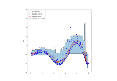
Prediction Intervals for Gradient Boosting Regression
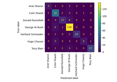
Faces recognition example using eigenfaces and SVMs
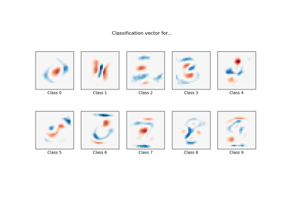
MNIST classification using multinomial logistic + L1
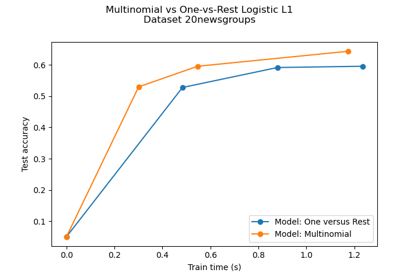
Multiclass sparse logistic regression on 20newgroups
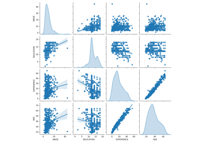
Common pitfalls in the interpretation of coefficients of linear models
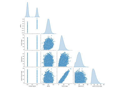
Failure of Machine Learning to infer causal effects
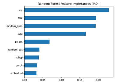
Permutation Importance vs Random Forest Feature Importance (MDI)
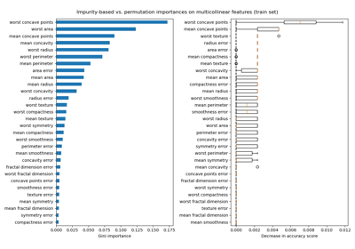
Permutation Importance with Multicollinear or Correlated Features
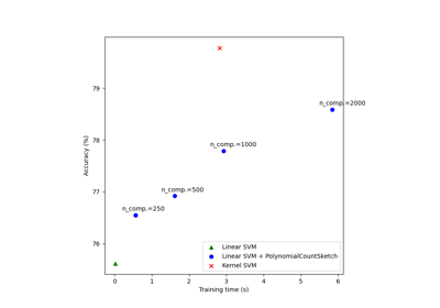
Scalable learning with polynomial kernel approximation
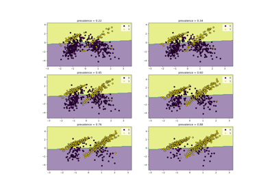
Class Likelihood Ratios to measure classification performance

Custom refit strategy of a grid search with cross-validation
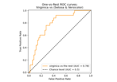
Multiclass Receiver Operating Characteristic (ROC)
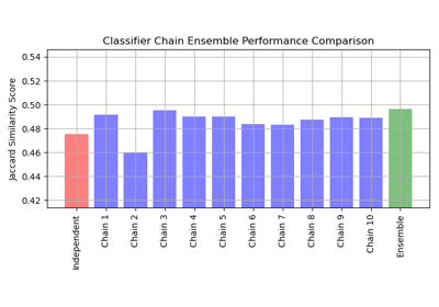
Multilabel classification using a classifier chain
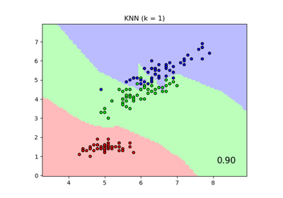
Comparing Nearest Neighbors with and without Neighborhood Components Analysis
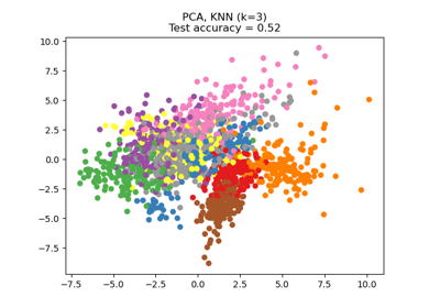
Dimensionality Reduction with Neighborhood Components Analysis
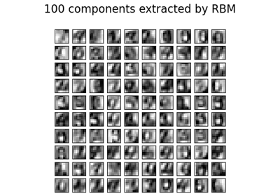
Restricted Boltzmann Machine features for digit classification
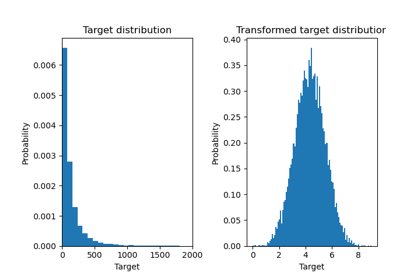
Effect of transforming the targets in regression model
