Note
Go to the end to download the full example code or to run this example in your browser via JupyterLite or Binder
Early stopping in Gradient Boosting
Gradient Boosting is an ensemble technique that combines multiple weak learners, typically decision trees, to create a robust and powerful predictive model. It does so in an iterative fashion, where each new stage (tree) corrects the errors of the previous ones.
Early stopping is a technique in Gradient Boosting that allows us to find
the optimal number of iterations required to build a model that generalizes
well to unseen data and avoids overfitting. The concept is simple: we set
aside a portion of our dataset as a validation set (specified using
validation_fraction) to assess the model’s performance during training.
As the model is iteratively built with additional stages (trees), its
performance on the validation set is monitored as a function of the
number of steps.
Early stopping becomes effective when the model’s performance on the
validation set plateaus or worsens (within deviations specified by tol)
over a certain number of consecutive stages (specified by n_iter_no_change).
This signals that the model has reached a point where further iterations may
lead to overfitting, and it’s time to stop training.
The number of estimators (trees) in the final model, when early stopping is
applied, can be accessed using the n_estimators_ attribute. Overall, early
stopping is a valuable tool to strike a balance between model performance and
efficiency in gradient boosting.
License: BSD 3 clause
Data Preparation
First we load and prepares the California Housing Prices dataset for training and evaluation. It subsets the dataset, splits it into training and validation sets.
import time

import matplotlib.pyplot as plt

from sklearn.datasets import fetch_california_housing
from sklearn.ensemble import GradientBoostingRegressor
from sklearn.metrics import mean_squared_error
from sklearn.model_selection import train_test_split

data = fetch_california_housing()
X, y = data.data[:600], data.target[:600]

X_train, X_val, y_train, y_val = train_test_split(X, y, test_size=0.2, random_state=42)
Model Training and Comparison
Two GradientBoostingRegressor models are trained:
one with and another without early stopping. The purpose is to compare their
performance. It also calculates the training time and the n_estimators_
used by both models.
params = dict(n_estimators=1000, max_depth=5, learning_rate=0.1, random_state=42)

gbm_full = GradientBoostingRegressor(**params)
gbm_early_stopping = GradientBoostingRegressor(
    **params,
    validation_fraction=0.1,
    n_iter_no_change=10,
)

start_time = time.time()
gbm_full.fit(X_train, y_train)
training_time_full = time.time() - start_time
n_estimators_full = gbm_full.n_estimators_

start_time = time.time()
gbm_early_stopping.fit(X_train, y_train)
training_time_early_stopping = time.time() - start_time
estimators_early_stopping = gbm_early_stopping.n_estimators_
Error Calculation
The code calculates the mean_squared_error for both
training and validation datasets for the models trained in the previous
section. It computes the errors for each boosting iteration. The purpose is
to assess the performance and convergence of the models.
train_errors_without = []
val_errors_without = []

train_errors_with = []
val_errors_with = []

for i, (train_pred, val_pred) in enumerate(
    zip(
        gbm_full.staged_predict(X_train),
        gbm_full.staged_predict(X_val),
    )
):
    train_errors_without.append(mean_squared_error(y_train, train_pred))
    val_errors_without.append(mean_squared_error(y_val, val_pred))

for i, (train_pred, val_pred) in enumerate(
    zip(
        gbm_early_stopping.staged_predict(X_train),
        gbm_early_stopping.staged_predict(X_val),
    )
):
    train_errors_with.append(mean_squared_error(y_train, train_pred))
    val_errors_with.append(mean_squared_error(y_val, val_pred))
Visualize Comparison
It includes three subplots:
Plotting training errors of both models over boosting iterations.
Plotting validation errors of both models over boosting iterations.
Creating a bar chart to compare the training times and the estimator used of the models with and without early stopping.
fig, axes = plt.subplots(ncols=3, figsize=(12, 4))

axes[0].plot(train_errors_without, label="gbm_full")
axes[0].plot(train_errors_with, label="gbm_early_stopping")
axes[0].set_xlabel("Boosting Iterations")
axes[0].set_ylabel("MSE (Training)")
axes[0].set_yscale("log")
axes[0].legend()
axes[0].set_title("Training Error")

axes[1].plot(val_errors_without, label="gbm_full")
axes[1].plot(val_errors_with, label="gbm_early_stopping")
axes[1].set_xlabel("Boosting Iterations")
axes[1].set_ylabel("MSE (Validation)")
axes[1].set_yscale("log")
axes[1].legend()
axes[1].set_title("Validation Error")

training_times = [training_time_full, training_time_early_stopping]
labels = ["gbm_full", "gbm_early_stopping"]
bars = axes[2].bar(labels, training_times)
axes[2].set_ylabel("Training Time (s)")

for bar, n_estimators in zip(bars, [n_estimators_full, estimators_early_stopping]):
    height = bar.get_height()
    axes[2].text(
        bar.get_x() + bar.get_width() / 2,
        height + 0.001,
        f"Estimators: {n_estimators}",
        ha="center",
        va="bottom",
    )

plt.tight_layout()
plt.show()
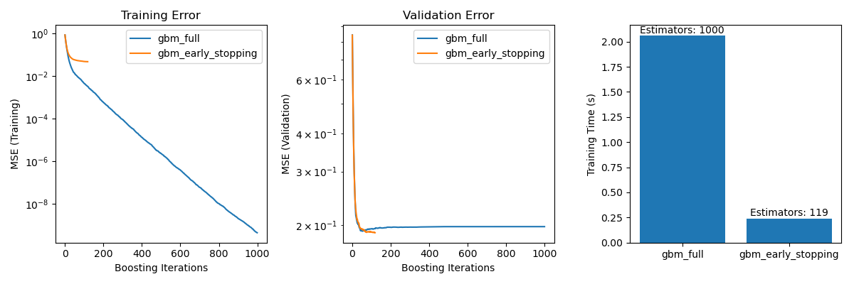
The difference in training error between the gbm_full and the
gbm_early_stopping stems from the fact that gbm_early_stopping sets
aside validation_fraction of the training data as internal validation set.
Early stopping is decided based on this internal validation score.
Summary
In our example with the GradientBoostingRegressor
model on the California Housing Prices dataset, we have demonstrated the
practical benefits of early stopping:
Preventing Overfitting: We showed how the validation error stabilizes or starts to increase after a certain point, indicating that the model generalizes better to unseen data. This is achieved by stopping the training process before overfitting occurs.
Improving Training Efficiency: We compared training times between models with and without early stopping. The model with early stopping achieved comparable accuracy while requiring significantly fewer estimators, resulting in faster training.
Total running time of the script: (0 minutes 3.297 seconds)
Related examples

Comparing Random Forests and Histogram Gradient Boosting models
