This is documentation for an old release of Scikit-learn (version 1.4). Try the latest stable release (version 1.6) or development (unstable) versions.

Note

Go to the end to download the full example code or to run this example in your browser via JupyterLite or Binder

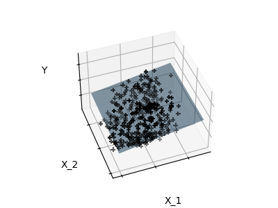
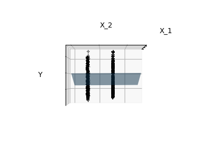
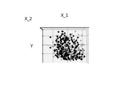
Sparsity Example: Fitting only features 1 and 2¶

Features 1 and 2 of the diabetes-dataset are fitted and plotted below. It illustrates that although feature 2 has a strong coefficient on the full model, it does not give us much regarding y when compared to just feature 1.

# Code source: Gaël Varoquaux
# Modified for documentation by Jaques Grobler
# License: BSD 3 clause

First we load the diabetes dataset.

import numpy as np

from sklearn import datasets

X, y = datasets.load_diabetes(return_X_y=True)
indices = (0, 1)

X_train = X[:-20, indices]
X_test = X[-20:, indices]
y_train = y[:-20]
y_test = y[-20:]

Next we fit a linear regression model.

from sklearn import linear_model

ols = linear_model.LinearRegression()
_ = ols.fit(X_train, y_train)

Finally we plot the figure from three different views.

import matplotlib.pyplot as plt

# unused but required import for doing 3d projections with matplotlib < 3.2
import mpl_toolkits.mplot3d  # noqa: F401


def plot_figs(fig_num, elev, azim, X_train, clf):
    fig = plt.figure(fig_num, figsize=(4, 3))
    plt.clf()
    ax = fig.add_subplot(111, projection="3d", elev=elev, azim=azim)

    ax.scatter(X_train[:, 0], X_train[:, 1], y_train, c="k", marker="+")
    ax.plot_surface(
        np.array([[-0.1, -0.1], [0.15, 0.15]]),
        np.array([[-0.1, 0.15], [-0.1, 0.15]]),
        clf.predict(
            np.array([[-0.1, -0.1, 0.15, 0.15], [-0.1, 0.15, -0.1, 0.15]]).T
        ).reshape((2, 2)),
        alpha=0.5,
    )
    ax.set_xlabel("X_1")
    ax.set_ylabel("X_2")
    ax.set_zlabel("Y")
    ax.xaxis.set_ticklabels([])
    ax.yaxis.set_ticklabels([])
    ax.zaxis.set_ticklabels([])


# Generate the three different figures from different views
elev = 43.5
azim = -110
plot_figs(1, elev, azim, X_train, ols)

elev = -0.5
azim = 0
plot_figs(2, elev, azim, X_train, ols)

elev = -0.5
azim = 90
plot_figs(3, elev, azim, X_train, ols)

plt.show()