Release Highlights for scikit-learn 1.0

We are very pleased to announce the release of scikit-learn 1.0! The library has been stable for quite some time, releasing version 1.0 is recognizing that and signalling it to our users. This release does not include any breaking changes apart from the usual two-release deprecation cycle. For the future, we do our best to keep this pattern.

This release includes some new key features as well as many improvements and bug fixes. We detail below a few of the major features of this release. For an exhaustive list of all the changes, please refer to the release notes.

To install the latest version (with pip):

pip install --upgrade scikit-learn

or with conda:

conda install -c conda-forge scikit-learn

Keyword and positional arguments

The scikit-learn API exposes many functions and methods which have many input parameters. For example, before this release, one could instantiate a HistGradientBoostingRegressor as:

HistGradientBoostingRegressor("squared_error", 0.1, 100, 31, None,
    20, 0.0, 255, None, None, False, "auto", "loss", 0.1, 10, 1e-7,
    0, None)

Understanding the above code requires the reader to go to the API documentation and to check each and every parameter for its position and its meaning. To improve the readability of code written based on scikit-learn, now users have to provide most parameters with their names, as keyword arguments, instead of positional arguments. For example, the above code would be:

HistGradientBoostingRegressor(
    loss="squared_error",
    learning_rate=0.1,
    max_iter=100,
    max_leaf_nodes=31,
    max_depth=None,
    min_samples_leaf=20,
    l2_regularization=0.0,
    max_bins=255,
    categorical_features=None,
    monotonic_cst=None,
    warm_start=False,
    early_stopping="auto",
    scoring="loss",
    validation_fraction=0.1,
    n_iter_no_change=10,
    tol=1e-7,
    verbose=0,
    random_state=None,
)

which is much more readable. Positional arguments have been deprecated since version 0.23 and will now raise a TypeError. A limited number of positional arguments are still allowed in some cases, for example in PCA, where PCA(10) is still allowed, but PCA(10, False) is not allowed.

Spline Transformers

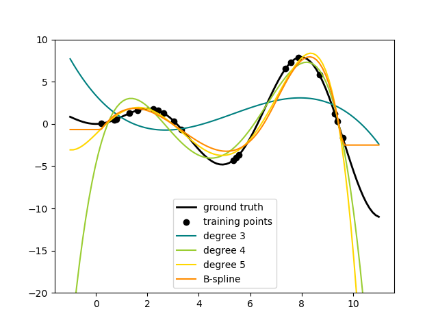
One way to add nonlinear terms to a dataset’s feature set is to generate spline basis functions for continuous/numerical features with the new SplineTransformer. Splines are piecewise polynomials, parametrized by their polynomial degree and the positions of the knots. The SplineTransformer implements a B-spline basis.

The following code shows splines in action, for more information, please refer to the User Guide.

import numpy as np
from sklearn.preprocessing import SplineTransformer

X = np.arange(5).reshape(5, 1)
spline = SplineTransformer(degree=2, n_knots=3)
spline.fit_transform(X)

array([[0.5  , 0.5  , 0.   , 0.   ],
       [0.125, 0.75 , 0.125, 0.   ],
       [0.   , 0.5  , 0.5  , 0.   ],
       [0.   , 0.125, 0.75 , 0.125],
       [0.   , 0.   , 0.5  , 0.5  ]])

Quantile Regressor

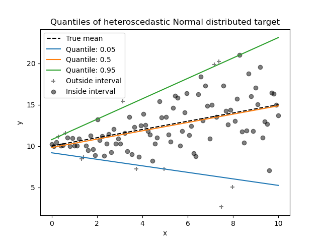
Quantile regression estimates the median or other quantiles of \(y\) conditional on \(X\), while ordinary least squares (OLS) estimates the conditional mean.

As a linear model, the new QuantileRegressor gives linear predictions \(\hat{y}(w, X) = Xw\) for the \(q\)-th quantile, \(q \in (0, 1)\). The weights or coefficients \(w\) are then found by the following minimization problem:

\[\min_{w} {\frac{1}{n_{\text{samples}}} \sum_i PB_q(y_i - X_i w) + \alpha ||w||_1}.\]

This consists of the pinball loss (also known as linear loss), see also mean_pinball_loss,

\[\begin{split}PB_q(t) = q \max(t, 0) + (1 - q) \max(-t, 0) = \begin{cases} q t, & t > 0, \\ 0, & t = 0, \\ (1-q) t, & t < 0 \end{cases}\end{split}\]

and the L1 penalty controlled by parameter alpha, similar to linear_model.Lasso.

Please check the following example to see how it works, and the User Guide for more details.

Feature Names Support

When an estimator is passed a pandas’ dataframe during fit, the estimator will set a feature_names_in_ attribute containing the feature names. Note that feature names support is only enabled when the column names in the dataframe are all strings. feature_names_in_ is used to check that the column names of the dataframe passed in non-fit, such as predict, are consistent with features in fit:

from sklearn.preprocessing import StandardScaler
import pandas as pd

X = pd.DataFrame([[1, 2, 3], [4, 5, 6]], columns=["a", "b", "c"])
scalar = StandardScaler().fit(X)
scalar.feature_names_in_

array(['a', 'b', 'c'], dtype=object)

The support of get_feature_names_out is available for transformers that already had get_feature_names and transformers with a one-to-one correspondence between input and output such as StandardScaler. get_feature_names_out support will be added to all other transformers in future releases. Additionally, compose.ColumnTransformer.get_feature_names_out is available to combine feature names of its transformers:

from sklearn.compose import ColumnTransformer
from sklearn.preprocessing import OneHotEncoder
import pandas as pd

X = pd.DataFrame({"pet": ["dog", "cat", "fish"], "age": [3, 7, 1]})
preprocessor = ColumnTransformer(
    [
        ("numerical", StandardScaler(), ["age"]),
        ("categorical", OneHotEncoder(), ["pet"]),
    ],
    verbose_feature_names_out=False,
).fit(X)

preprocessor.get_feature_names_out()

array(['age', 'pet_cat', 'pet_dog', 'pet_fish'], dtype=object)

When this preprocessor is used with a pipeline, the feature names used by the classifier are obtained by slicing and calling get_feature_names_out:

from sklearn.linear_model import LogisticRegression
from sklearn.pipeline import make_pipeline

y = [1, 0, 1]
pipe = make_pipeline(preprocessor, LogisticRegression())
pipe.fit(X, y)
pipe[:-1].get_feature_names_out()

array(['age', 'pet_cat', 'pet_dog', 'pet_fish'], dtype=object)

A more flexible plotting API

metrics.ConfusionMatrixDisplay, metrics.PrecisionRecallDisplay, metrics.DetCurveDisplay, and inspection.PartialDependenceDisplay now expose two class methods: from_estimator and from_predictions which allow users to create a plot given the predictions or an estimator. This means the corresponding plot_* functions are deprecated. Please check example one and example two for how to use the new plotting functionalities.

Online One-Class SVM

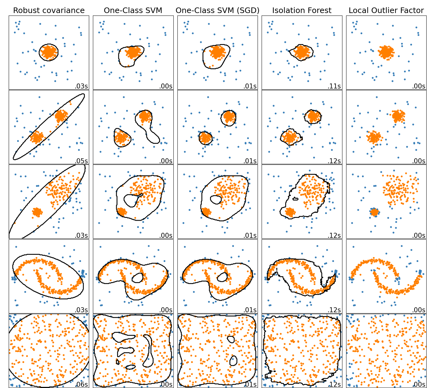
The new class SGDOneClassSVM implements an online linear version of the One-Class SVM using a stochastic gradient descent. Combined with kernel approximation techniques, SGDOneClassSVM can be used to approximate the solution of a kernelized One-Class SVM, implemented in OneClassSVM, with a fit time complexity linear in the number of samples. Note that the complexity of a kernelized One-Class SVM is at best quadratic in the number of samples. SGDOneClassSVM is thus well suited for datasets with a large number of training samples (> 10,000) for which the SGD variant can be several orders of magnitude faster. Please check this example to see how it’s used, and the User Guide for more details.

Histogram-based Gradient Boosting Models are now stable

HistGradientBoostingRegressor and HistGradientBoostingClassifier are no longer experimental and can simply be imported and used as:

from sklearn.ensemble import HistGradientBoostingClassifier

New documentation improvements

This release includes many documentation improvements. Out of over 2100 merged pull requests, about 800 of them are improvements to our documentation.