Note
Click here to download the full example code or to run this example in your browser via Binder
Release Highlights for scikit-learn 1.1
We are pleased to announce the release of scikit-learn 1.1! Many bug fixes and improvements were added, as well as some new key features. We detail below a few of the major features of this release. For an exhaustive list of all the changes, please refer to the release notes.
To install the latest version (with pip):
pip install --upgrade scikit-learn
or with conda:
conda install -c conda-forge scikit-learn
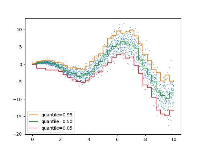
Quantile loss in ensemble.HistGradientBoostingRegressor
ensemble.HistGradientBoostingRegressor can model quantiles with
loss="quantile" and the new parameter quantile.
from sklearn.ensemble import HistGradientBoostingRegressor
import numpy as np
import matplotlib.pyplot as plt

# Simple regression function for X * cos(X)
rng = np.random.RandomState(42)
X_1d = np.linspace(0, 10, num=2000)
X = X_1d.reshape(-1, 1)
y = X_1d * np.cos(X_1d) + rng.normal(scale=X_1d / 3)

quantiles = [0.95, 0.5, 0.05]
parameters = dict(loss="quantile", max_bins=32, max_iter=50)
hist_quantiles = {
    f"quantile={quantile:.2f}": HistGradientBoostingRegressor(
        **parameters, quantile=quantile
    ).fit(X, y)
    for quantile in quantiles
}

fig, ax = plt.subplots()
ax.plot(X_1d, y, "o", alpha=0.5, markersize=1)
for quantile, hist in hist_quantiles.items():
    ax.plot(X_1d, hist.predict(X), label=quantile)
_ = ax.legend(loc="lower left")
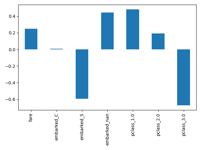
get_feature_names_out Available in all Transformers
get_feature_names_out is now available in all Transformers. This enables
pipeline.Pipeline to construct the output feature names for more complex
pipelines:
from sklearn.compose import ColumnTransformer
from sklearn.preprocessing import OneHotEncoder, StandardScaler
from sklearn.pipeline import make_pipeline
from sklearn.impute import SimpleImputer
from sklearn.feature_selection import SelectKBest
from sklearn.datasets import fetch_openml
from sklearn.linear_model import LogisticRegression

X, y = fetch_openml("titanic", version=1, as_frame=True, return_X_y=True)
numeric_features = ["age", "fare"]
numeric_transformer = make_pipeline(SimpleImputer(strategy="median"), StandardScaler())
categorical_features = ["embarked", "pclass"]

preprocessor = ColumnTransformer(
    [
        ("num", numeric_transformer, numeric_features),
        (
            "cat",
            OneHotEncoder(handle_unknown="ignore", sparse=False),
            categorical_features,
        ),
    ],
    verbose_feature_names_out=False,
)
log_reg = make_pipeline(preprocessor, SelectKBest(k=7), LogisticRegression())
log_reg.fit(X, y)
Here we slice the pipeline to include all the steps but the last one. The output feature names of this pipeline slice are the features put into logistic regression. These names correspond directly to the coefficients in the logistic regression:
import pandas as pd

log_reg_input_features = log_reg[:-1].get_feature_names_out()
pd.Series(log_reg[-1].coef_.ravel(), index=log_reg_input_features).plot.bar()
plt.tight_layout()
Grouping infrequent categories in OneHotEncoder
OneHotEncoder supports aggregating infrequent categories into a single
output for each feature. The parameters to enable the gathering of infrequent
categories are min_frequency and max_categories. See the
User Guide for more details.
from sklearn.preprocessing import OneHotEncoder
import numpy as np

X = np.array(
    [["dog"] * 5 + ["cat"] * 20 + ["rabbit"] * 10 + ["snake"] * 3], dtype=object
).T
enc = OneHotEncoder(min_frequency=6, sparse=False).fit(X)
enc.infrequent_categories_
[array(['dog', 'snake'], dtype=object)]
Since dog and snake are infrequent categories, they are grouped together when transformed:
encoded = enc.transform(np.array([["dog"], ["snake"], ["cat"], ["rabbit"]]))
pd.DataFrame(encoded, columns=enc.get_feature_names_out())
Performance improvements
Reductions on pairwise distances for dense float64 datasets has been refactored
to better take advantage of non-blocking thread parallelism. For example,
neighbors.NearestNeighbors.kneighbors and
neighbors.NearestNeighbors.radius_neighbors can respectively be up to ×20 and
×5 faster than previously. In summary, the following functions and estimators
now benefit from improved performance:
To know more about the technical details of this work, you can read this suite of blog posts.
Moreover, the computation of loss functions has been refactored using Cython resulting in performance improvements for the following estimators:
MiniBatchNMF: an online version of NMF
The new class decomposition.MiniBatchNMF implements a faster but less
accurate version of non-negative matrix factorization (decomposition.NMF).
MiniBatchNMF divides the data into mini-batches and optimizes the NMF model
in an online manner by cycling over the mini-batches, making it better suited for
large datasets. In particular, it implements partial_fit, which can be used for
online learning when the data is not readily available from the start, or when the
data does not fit into memory.
import numpy as np
from sklearn.decomposition import MiniBatchNMF

rng = np.random.RandomState(0)
n_samples, n_features, n_components = 10, 10, 5
true_W = rng.uniform(size=(n_samples, n_components))
true_H = rng.uniform(size=(n_components, n_features))
X = true_W @ true_H

nmf = MiniBatchNMF(n_components=n_components, random_state=0)

for _ in range(10):
    nmf.partial_fit(X)

W = nmf.transform(X)
H = nmf.components_
X_reconstructed = W @ H

print(
    f"relative reconstruction error: ",
    f"{np.sum((X - X_reconstructed) ** 2) / np.sum(X**2):.5f}",
)
relative reconstruction error: 0.00364
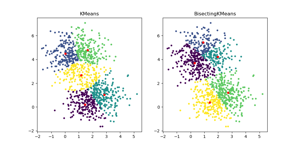
BisectingKMeans: divide and cluster
The new class cluster.BisectingKMeans is a variant of KMeans, using
divisive hierarchical clustering. Instead of creating all centroids at once, centroids
are picked progressively based on a previous clustering: a cluster is split into two
new clusters repeatedly until the target number of clusters is reached, giving a
hierarchical structure to the clustering.
from sklearn.datasets import make_blobs
from sklearn.cluster import KMeans, BisectingKMeans
import matplotlib.pyplot as plt

X, _ = make_blobs(n_samples=1000, centers=2, random_state=0)

km = KMeans(n_clusters=5, random_state=0).fit(X)
bisect_km = BisectingKMeans(n_clusters=5, random_state=0).fit(X)

fig, ax = plt.subplots(1, 2, figsize=(10, 5))
ax[0].scatter(X[:, 0], X[:, 1], s=10, c=km.labels_)
ax[0].scatter(km.cluster_centers_[:, 0], km.cluster_centers_[:, 1], s=20, c="r")
ax[0].set_title("KMeans")

ax[1].scatter(X[:, 0], X[:, 1], s=10, c=bisect_km.labels_)
ax[1].scatter(
    bisect_km.cluster_centers_[:, 0], bisect_km.cluster_centers_[:, 1], s=20, c="r"
)
_ = ax[1].set_title("BisectingKMeans")
Total running time of the script: ( 0 minutes 9.704 seconds)