sklearn.preprocessing.StandardScaler
- class sklearn.preprocessing.StandardScaler(*, copy=True, with_mean=True, with_std=True)[source]
Standardize features by removing the mean and scaling to unit variance.
The standard score of a sample
xis calculated as:z = (x - u) / s
where
uis the mean of the training samples or zero ifwith_mean=False, andsis the standard deviation of the training samples or one ifwith_std=False.Centering and scaling happen independently on each feature by computing the relevant statistics on the samples in the training set. Mean and standard deviation are then stored to be used on later data using
transform.Standardization of a dataset is a common requirement for many machine learning estimators: they might behave badly if the individual features do not more or less look like standard normally distributed data (e.g. Gaussian with 0 mean and unit variance).
For instance many elements used in the objective function of a learning algorithm (such as the RBF kernel of Support Vector Machines or the L1 and L2 regularizers of linear models) assume that all features are centered around 0 and have variance in the same order. If a feature has a variance that is orders of magnitude larger than others, it might dominate the objective function and make the estimator unable to learn from other features correctly as expected.
This scaler can also be applied to sparse CSR or CSC matrices by passing
with_mean=Falseto avoid breaking the sparsity structure of the data.Read more in the User Guide.
- Parameters:
- copybool, default=True
If False, try to avoid a copy and do inplace scaling instead. This is not guaranteed to always work inplace; e.g. if the data is not a NumPy array or scipy.sparse CSR matrix, a copy may still be returned.
- with_meanbool, default=True
If True, center the data before scaling. This does not work (and will raise an exception) when attempted on sparse matrices, because centering them entails building a dense matrix which in common use cases is likely to be too large to fit in memory.
- with_stdbool, default=True
If True, scale the data to unit variance (or equivalently, unit standard deviation).
- Attributes:
- scale_ndarray of shape (n_features,) or None
Per feature relative scaling of the data to achieve zero mean and unit variance. Generally this is calculated using
np.sqrt(var_). If a variance is zero, we can’t achieve unit variance, and the data is left as-is, giving a scaling factor of 1.scale_is equal toNonewhenwith_std=False.New in version 0.17: scale_
- mean_ndarray of shape (n_features,) or None
The mean value for each feature in the training set. Equal to
Nonewhenwith_mean=False.- var_ndarray of shape (n_features,) or None
The variance for each feature in the training set. Used to compute
scale_. Equal toNonewhenwith_std=False.- n_features_in_int
Number of features seen during fit.
New in version 0.24.
- feature_names_in_ndarray of shape (
n_features_in_,) Names of features seen during fit. Defined only when
Xhas feature names that are all strings.New in version 1.0.
- n_samples_seen_int or ndarray of shape (n_features,)
The number of samples processed by the estimator for each feature. If there are no missing samples, the
n_samples_seenwill be an integer, otherwise it will be an array of dtype int. Ifsample_weightsare used it will be a float (if no missing data) or an array of dtype float that sums the weights seen so far. Will be reset on new calls to fit, but increments acrosspartial_fitcalls.
See also
Notes
NaNs are treated as missing values: disregarded in fit, and maintained in transform.
We use a biased estimator for the standard deviation, equivalent to
numpy.std(x, ddof=0). Note that the choice ofddofis unlikely to affect model performance.For a comparison of the different scalers, transformers, and normalizers, see examples/preprocessing/plot_all_scaling.py.
Examples
>>> from sklearn.preprocessing import StandardScaler
>>> data = [[0, 0], [0, 0], [1, 1], [1, 1]]
>>> scaler = StandardScaler()
>>> print(scaler.fit(data))
StandardScaler()
>>> print(scaler.mean_)
[0.5 0.5]
>>> print(scaler.transform(data))
[[-1. -1.]
 [-1. -1.]
 [ 1.  1.]
 [ 1.  1.]]
>>> print(scaler.transform([[2, 2]]))
[[3. 3.]]
Methods
fit(X[, y, sample_weight])Compute the mean and std to be used for later scaling.
fit_transform(X[, y])Fit to data, then transform it.
get_feature_names_out([input_features])Get output feature names for transformation.
get_params([deep])Get parameters for this estimator.
inverse_transform(X[, copy])Scale back the data to the original representation.
partial_fit(X[, y, sample_weight])Online computation of mean and std on X for later scaling.
set_output(*[, transform])Set output container.
set_params(**params)Set the parameters of this estimator.
transform(X[, copy])Perform standardization by centering and scaling.
- fit(X, y=None, sample_weight=None)[source]
Compute the mean and std to be used for later scaling.
- Parameters:
- X{array-like, sparse matrix} of shape (n_samples, n_features)
The data used to compute the mean and standard deviation used for later scaling along the features axis.
- yNone
Ignored.
- sample_weightarray-like of shape (n_samples,), default=None
Individual weights for each sample.
New in version 0.24: parameter sample_weight support to StandardScaler.
- Returns:
- selfobject
Fitted scaler.
- fit_transform(X, y=None, **fit_params)[source]
Fit to data, then transform it.
Fits transformer to
Xandywith optional parametersfit_paramsand returns a transformed version ofX.- Parameters:
- Xarray-like of shape (n_samples, n_features)
Input samples.
- yarray-like of shape (n_samples,) or (n_samples, n_outputs), default=None
Target values (None for unsupervised transformations).
- **fit_paramsdict
Additional fit parameters.
- Returns:
- X_newndarray array of shape (n_samples, n_features_new)
Transformed array.
- get_feature_names_out(input_features=None)[source]
Get output feature names for transformation.
- Parameters:
- input_featuresarray-like of str or None, default=None
Input features.
If
input_featuresisNone, thenfeature_names_in_is used as feature names in. Iffeature_names_in_is not defined, then the following input feature names are generated:["x0", "x1", ..., "x(n_features_in_ - 1)"].If
input_featuresis an array-like, theninput_featuresmust matchfeature_names_in_iffeature_names_in_is defined.
- Returns:
- feature_names_outndarray of str objects
Same as input features.
- get_params(deep=True)[source]
Get parameters for this estimator.
- Parameters:
- deepbool, default=True
If True, will return the parameters for this estimator and contained subobjects that are estimators.
- Returns:
- paramsdict
Parameter names mapped to their values.
- inverse_transform(X, copy=None)[source]
Scale back the data to the original representation.
- Parameters:
- X{array-like, sparse matrix} of shape (n_samples, n_features)
The data used to scale along the features axis.
- copybool, default=None
Copy the input X or not.
- Returns:
- X_tr{ndarray, sparse matrix} of shape (n_samples, n_features)
Transformed array.
- partial_fit(X, y=None, sample_weight=None)[source]
Online computation of mean and std on X for later scaling.
All of X is processed as a single batch. This is intended for cases when
fitis not feasible due to very large number ofn_samplesor because X is read from a continuous stream.The algorithm for incremental mean and std is given in Equation 1.5a,b in Chan, Tony F., Gene H. Golub, and Randall J. LeVeque. “Algorithms for computing the sample variance: Analysis and recommendations.” The American Statistician 37.3 (1983): 242-247:
- Parameters:
- X{array-like, sparse matrix} of shape (n_samples, n_features)
The data used to compute the mean and standard deviation used for later scaling along the features axis.
- yNone
Ignored.
- sample_weightarray-like of shape (n_samples,), default=None
Individual weights for each sample.
New in version 0.24: parameter sample_weight support to StandardScaler.
- Returns:
- selfobject
Fitted scaler.
- set_output(*, transform=None)[source]
Set output container.
See Introducing the set_output API for an example on how to use the API.
- Parameters:
- transform{“default”, “pandas”}, default=None
Configure output of
transformandfit_transform."default": Default output format of a transformer"pandas": DataFrame outputNone: Transform configuration is unchanged
- Returns:
- selfestimator instance
Estimator instance.
- set_params(**params)[source]
Set the parameters of this estimator.
The method works on simple estimators as well as on nested objects (such as
Pipeline). The latter have parameters of the form<component>__<parameter>so that it’s possible to update each component of a nested object.- Parameters:
- **paramsdict
Estimator parameters.
- Returns:
- selfestimator instance
Estimator instance.
- transform(X, copy=None)[source]
Perform standardization by centering and scaling.
- Parameters:
- X{array-like, sparse matrix of shape (n_samples, n_features)
The data used to scale along the features axis.
- copybool, default=None
Copy the input X or not.
- Returns:
- X_tr{ndarray, sparse matrix} of shape (n_samples, n_features)
Transformed array.
Examples using sklearn.preprocessing.StandardScaler

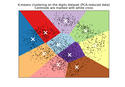
A demo of K-Means clustering on the handwritten digits data
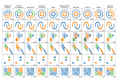
Comparing different clustering algorithms on toy datasets
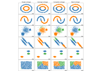
Comparing different hierarchical linkage methods on toy datasets
Principal Component Regression vs Partial Least Squares Regression
Factor Analysis (with rotation) to visualize patterns
Faces recognition example using eigenfaces and SVMs
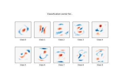
MNIST classification using multinomial logistic + L1
Common pitfalls in the interpretation of coefficients of linear models


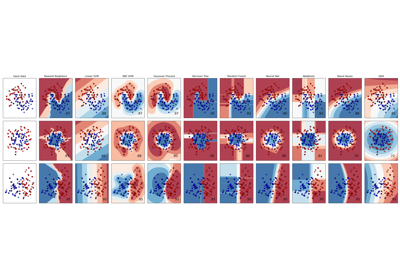
Comparing Nearest Neighbors with and without Neighborhood Components Analysis
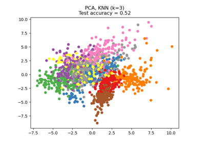
Dimensionality Reduction with Neighborhood Components Analysis

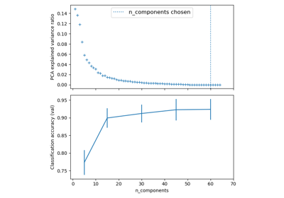
Pipelining: chaining a PCA and a logistic regression
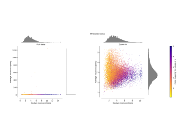
Compare the effect of different scalers on data with outliers