Introducing the set_output API

This example will demonstrate the set_output API to configure transformers to output pandas DataFrames. set_output can be configured per estimator by calling the set_output method or globally by setting set_config(transform_output="pandas"). For details, see SLEP018.

First, we load the iris dataset as a DataFrame to demonstrate the set_output API.

from sklearn.datasets import load_iris
from sklearn.model_selection import train_test_split

X, y = load_iris(as_frame=True, return_X_y=True)
X_train, X_test, y_train, y_test = train_test_split(X, y, stratify=y, random_state=0)
X_train.head()

	sepal length (cm)	sepal width (cm)	petal length (cm)	petal width (cm)
60	5.0	2.0	3.5	1.0
1	4.9	3.0	1.4	0.2
8	4.4	2.9	1.4	0.2
93	5.0	2.3	3.3	1.0
106	4.9	2.5	4.5	1.7

To configure an estimator such as preprocessing.StandardScaler to return DataFrames, call set_output. This feature requires pandas to be installed.

from sklearn.preprocessing import StandardScaler

scaler = StandardScaler().set_output(transform="pandas")

scaler.fit(X_train)
X_test_scaled = scaler.transform(X_test)
X_test_scaled.head()

	sepal length (cm)	sepal width (cm)	petal length (cm)	petal width (cm)
39	-0.894264	0.798301	-1.271411	-1.327605
12	-1.244466	-0.086944	-1.327407	-1.459074
48	-0.660797	1.462234	-1.271411	-1.327605
23	-0.894264	0.576989	-1.159419	-0.933197
81	-0.427329	-1.414810	-0.039497	-0.275851

set_output can be called after fit to configure transform after the fact.

scaler2 = StandardScaler()

scaler2.fit(X_train)
X_test_np = scaler2.transform(X_test)
print(f"Default output type: {type(X_test_np).__name__}")

scaler2.set_output(transform="pandas")
X_test_df = scaler2.transform(X_test)
print(f"Configured pandas output type: {type(X_test_df).__name__}")

Default output type: ndarray
Configured pandas output type: DataFrame

In a pipeline.Pipeline, set_output configures all steps to output DataFrames.

from sklearn.pipeline import make_pipeline
from sklearn.linear_model import LogisticRegression
from sklearn.feature_selection import SelectPercentile

clf = make_pipeline(
    StandardScaler(), SelectPercentile(percentile=75), LogisticRegression()
)
clf.set_output(transform="pandas")
clf.fit(X_train, y_train)

Pipeline(steps=[('standardscaler', StandardScaler()),
                ('selectpercentile', SelectPercentile(percentile=75)),
                ('logisticregression', LogisticRegression())])

In a Jupyter environment, please rerun this cell to show the HTML representation or trust the notebook.
On GitHub, the HTML representation is unable to render, please try loading this page with nbviewer.org.

Each transformer in the pipeline is configured to return DataFrames. This means that the final logistic regression step contains the feature names of the input.

clf[-1].feature_names_in_

array(['sepal length (cm)', 'petal length (cm)', 'petal width (cm)'],
      dtype=object)

Next we load the titanic dataset to demonstrate set_output with compose.ColumnTransformer and heterogenous data.

from sklearn.datasets import fetch_openml

X, y = fetch_openml(
    "titanic", version=1, as_frame=True, return_X_y=True, parser="pandas"
)
X_train, X_test, y_train, y_test = train_test_split(X, y, stratify=y)

The set_output API can be configured globally by using set_config and setting transform_output to "pandas".

from sklearn.compose import ColumnTransformer
from sklearn.preprocessing import OneHotEncoder, StandardScaler
from sklearn.impute import SimpleImputer
from sklearn import set_config

set_config(transform_output="pandas")

num_pipe = make_pipeline(SimpleImputer(), StandardScaler())
num_cols = ["age", "fare"]
ct = ColumnTransformer(
    (
        ("numerical", num_pipe, num_cols),
        (
            "categorical",
            OneHotEncoder(
                sparse_output=False, drop="if_binary", handle_unknown="ignore"
            ),
            ["embarked", "sex", "pclass"],
        ),
    ),
    verbose_feature_names_out=False,
)
clf = make_pipeline(ct, SelectPercentile(percentile=50), LogisticRegression())
clf.fit(X_train, y_train)
clf.score(X_test, y_test)

0.7621951219512195

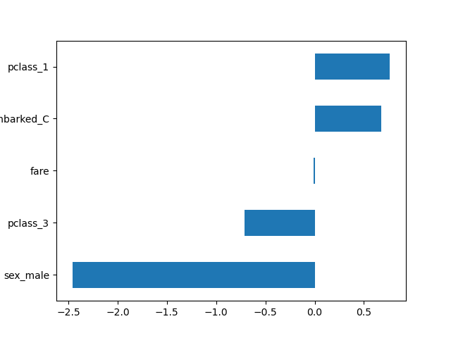
With the global configuration, all transformers output DataFrames. This allows us to easily plot the logistic regression coefficients with the corresponding feature names.

import pandas as pd

log_reg = clf[-1]
coef = pd.Series(log_reg.coef_.ravel(), index=log_reg.feature_names_in_)
_ = coef.sort_values().plot.barh()

This resets transform_output to its default value to avoid impacting other examples when generating the scikit-learn documentation

set_config(transform_output="default")

When configuring the output type with config_context the configuration at the time when transform or fit_transform are called is what counts. Setting these only when you construct or fit the transformer has no effect.

from sklearn import config_context

scaler = StandardScaler()
scaler.fit(X_train[num_cols])

StandardScaler()

In a Jupyter environment, please rerun this cell to show the HTML representation or trust the notebook.
On GitHub, the HTML representation is unable to render, please try loading this page with nbviewer.org.

with config_context(transform_output="pandas"):
    # the output of transform will be a Pandas DataFrame
    X_test_scaled = scaler.transform(X_test[num_cols])
X_test_scaled.head()

	age	fare
334	-0.133660	-0.438059
885	-0.894273	-0.506893
478	-2.000619	0.182778
671	-0.548540	-0.461032
817	-0.548540	-0.487001

outside of the context manager, the output will be a NumPy array

X_test_scaled = scaler.transform(X_test[num_cols])
X_test_scaled[:5]

array([[-0.13366001, -0.4380594 ],
       [-0.89427284, -0.50689261],
       [-2.00061876,  0.18277786],
       [-0.54853974, -0.46103177],
       [-0.54853974, -0.48700054]])