`sklearn.linear_model`.SGDRegressor¶

class sklearn.linear_model.SGDRegressor(loss='squared_error', *, penalty='l2', alpha=0.0001, l1_ratio=0.15, fit_intercept=True, max_iter=1000, tol=0.001, shuffle=True, verbose=0, epsilon=0.1, random_state=None, learning_rate='invscaling', eta0=0.01, power_t=0.25, early_stopping=False, validation_fraction=0.1, n_iter_no_change=5, warm_start=False, average=False)[source]¶

Linear model fitted by minimizing a regularized empirical loss with SGD.

SGD stands for Stochastic Gradient Descent: the gradient of the loss is estimated each sample at a time and the model is updated along the way with a decreasing strength schedule (aka learning rate).

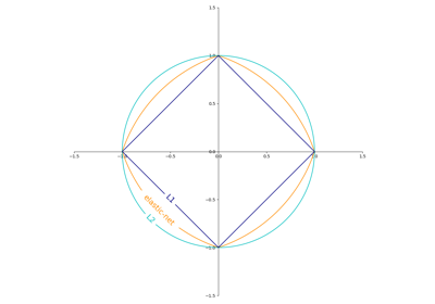
The regularizer is a penalty added to the loss function that shrinks model parameters towards the zero vector using either the squared euclidean norm L2 or the absolute norm L1 or a combination of both (Elastic Net). If the parameter update crosses the 0.0 value because of the regularizer, the update is truncated to 0.0 to allow for learning sparse models and achieve online feature selection.

This implementation works with data represented as dense numpy arrays of floating point values for the features.

See also

HuberRegressor: Linear regression model that is robust to outliers.
Lars: Least Angle Regression model.
Lasso: Linear Model trained with L1 prior as regularizer.
RANSACRegressor: RANSAC (RANdom SAmple Consensus) algorithm.
Ridge: Linear least squares with l2 regularization.
sklearn.svm.SVR: Epsilon-Support Vector Regression.
TheilSenRegressor: Theil-Sen Estimator robust multivariate regression model.

Examples

>>> import numpy as np
>>> from sklearn.linear_model import SGDRegressor
>>> from sklearn.pipeline import make_pipeline
>>> from sklearn.preprocessing import StandardScaler
>>> n_samples, n_features = 10, 5
>>> rng = np.random.RandomState(0)
>>> y = rng.randn(n_samples)
>>> X = rng.randn(n_samples, n_features)
>>> # Always scale the input. The most convenient way is to use a pipeline.
>>> reg = make_pipeline(StandardScaler(),
...                     SGDRegressor(max_iter=1000, tol=1e-3))
>>> reg.fit(X, y)
Pipeline(steps=[('standardscaler', StandardScaler()),
                ('sgdregressor', SGDRegressor())])

Methods

`densify`()	Convert coefficient matrix to dense array format.
`fit`(X, y[, coef_init, intercept_init, ...])	Fit linear model with Stochastic Gradient Descent.
`get_params`([deep])	Get parameters for this estimator.
`partial_fit`(X, y[, sample_weight])	Perform one epoch of stochastic gradient descent on given samples.
`predict`(X)	Predict using the linear model.
`score`(X, y[, sample_weight])	Return the coefficient of determination of the prediction.
`set_params`(**params)	Set the parameters of this estimator.
`sparsify`()	Convert coefficient matrix to sparse format.

densify()[source]¶

Convert coefficient matrix to dense array format.

Converts the coef_ member (back) to a numpy.ndarray. This is the default format of coef_ and is required for fitting, so calling this method is only required on models that have previously been sparsified; otherwise, it is a no-op.

Returns:

self: Fitted estimator.

fit(X, y, coef_init=None, intercept_init=None, sample_weight=None)[source]¶

Fit linear model with Stochastic Gradient Descent.

Parameters:

X{array-like, sparse matrix}, shape (n_samples, n_features): Training data.
yndarray of shape (n_samples,): Target values.
coef_initndarray of shape (n_features,), default=None: The initial coefficients to warm-start the optimization.
intercept_initndarray of shape (1,), default=None: The initial intercept to warm-start the optimization.
sample_weightarray-like, shape (n_samples,), default=None: Weights applied to individual samples (1. for unweighted).

Returns:

selfobject: Fitted SGDRegressor estimator.

get_params(deep=True)[source]¶

Get parameters for this estimator.

Parameters:

deepbool, default=True: If True, will return the parameters for this estimator and contained subobjects that are estimators.

Returns:

paramsdict: Parameter names mapped to their values.

partial_fit(X, y, sample_weight=None)[source]¶

Perform one epoch of stochastic gradient descent on given samples.

Internally, this method uses max_iter = 1. Therefore, it is not guaranteed that a minimum of the cost function is reached after calling it once. Matters such as objective convergence and early stopping should be handled by the user.

Parameters:

X{array-like, sparse matrix}, shape (n_samples, n_features): Subset of training data.
ynumpy array of shape (n_samples,): Subset of target values.
sample_weightarray-like, shape (n_samples,), default=None: Weights applied to individual samples. If not provided, uniform weights are assumed.

Returns:

selfobject: Returns an instance of self.

predict(X)[source]¶

Predict using the linear model.

Parameters:

X{array-like, sparse matrix}, shape (n_samples, n_features): Input data.

Returns:

ndarray of shape (n_samples,): Predicted target values per element in X.

score(X, y, sample_weight=None)[source]¶

Return the coefficient of determination of the prediction.

The coefficient of determination \(R^2\) is defined as \((1 - \frac{u}{v})\), where \(u\) is the residual sum of squares ((y_true - y_pred)** 2).sum() and \(v\) is the total sum of squares ((y_true - y_true.mean()) ** 2).sum(). The best possible score is 1.0 and it can be negative (because the model can be arbitrarily worse). A constant model that always predicts the expected value of y, disregarding the input features, would get a \(R^2\) score of 0.0.

Parameters:

Xarray-like of shape (n_samples, n_features): Test samples. For some estimators this may be a precomputed kernel matrix or a list of generic objects instead with shape (n_samples, n_samples_fitted), where n_samples_fitted is the number of samples used in the fitting for the estimator.
yarray-like of shape (n_samples,) or (n_samples, n_outputs): True values for X.
sample_weightarray-like of shape (n_samples,), default=None: Sample weights.

Returns:

scorefloat: \(R^2\) of self.predict(X) w.r.t. y.

Notes

The \(R^2\) score used when calling score on a regressor uses multioutput='uniform_average' from version 0.23 to keep consistent with default value of r2_score. This influences the score method of all the multioutput regressors (except for MultiOutputRegressor).

set_params(**params)[source]¶

Set the parameters of this estimator.

The method works on simple estimators as well as on nested objects (such as Pipeline). The latter have parameters of the form <component>__<parameter> so that it’s possible to update each component of a nested object.

Parameters:

**paramsdict: Estimator parameters.

Returns:

selfestimator instance: Estimator instance.

sparsify()[source]¶

Convert coefficient matrix to sparse format.

Converts the coef_ member to a scipy.sparse matrix, which for L1-regularized models can be much more memory- and storage-efficient than the usual numpy.ndarray representation.

The intercept_ member is not converted.

Returns:

self: Fitted estimator.

Notes

For non-sparse models, i.e. when there are not many zeros in coef_, this may actually increase memory usage, so use this method with care. A rule of thumb is that the number of zero elements, which can be computed with (coef_ == 0).sum(), must be more than 50% for this to provide significant benefits.

After calling this method, further fitting with the partial_fit method (if any) will not work until you call densify.

Examples using `sklearn.linear_model.SGDRegressor`¶

Prediction Latency

SGD: Penalties

sklearn.linear_model.SGDRegressor¶

Examples using sklearn.linear_model.SGDRegressor¶

`sklearn.linear_model`.SGDRegressor¶

Examples using `sklearn.linear_model.SGDRegressor`¶