`sklearn.decomposition`.PCA¶

class sklearn.decomposition.PCA(n_components=None, *, copy=True, whiten=False, svd_solver='auto', tol=0.0, iterated_power='auto', n_oversamples=10, power_iteration_normalizer='auto', random_state=None)[source]¶

Principal component analysis (PCA).

Linear dimensionality reduction using Singular Value Decomposition of the data to project it to a lower dimensional space. The input data is centered but not scaled for each feature before applying the SVD.

It uses the LAPACK implementation of the full SVD or a randomized truncated SVD by the method of Halko et al. 2009, depending on the shape of the input data and the number of components to extract.

It can also use the scipy.sparse.linalg ARPACK implementation of the truncated SVD.

Notice that this class does not support sparse input. See TruncatedSVD for an alternative with sparse data.

Read more in the User Guide.

Parameters:

n_componentsint, float or ‘mle’, default=None

Number of components to keep. if n_components is not set all components are kept:

n_components == min(n_samples, n_features)

If n_components == 'mle' and svd_solver == 'full', Minka’s MLE is used to guess the dimension. Use of n_components == 'mle' will interpret svd_solver == 'auto' as svd_solver == 'full'.

If 0 < n_components < 1 and svd_solver == 'full', select the number of components such that the amount of variance that needs to be explained is greater than the percentage specified by n_components.

If svd_solver == 'arpack', the number of components must be strictly less than the minimum of n_features and n_samples.

Hence, the None case results in:

n_components == min(n_samples, n_features) - 1

copybool, default=True

If False, data passed to fit are overwritten and running fit(X).transform(X) will not yield the expected results, use fit_transform(X) instead.

whitenbool, default=False

When True (False by default) the components_ vectors are multiplied by the square root of n_samples and then divided by the singular values to ensure uncorrelated outputs with unit component-wise variances.

Whitening will remove some information from the transformed signal (the relative variance scales of the components) but can sometime improve the predictive accuracy of the downstream estimators by making their data respect some hard-wired assumptions.

svd_solver{‘auto’, ‘full’, ‘arpack’, ‘randomized’}, default=’auto’

If auto :: The solver is selected by a default policy based on X.shape and n_components: if the input data is larger than 500x500 and the number of components to extract is lower than 80% of the smallest dimension of the data, then the more efficient ‘randomized’ method is enabled. Otherwise the exact full SVD is computed and optionally truncated afterwards.
If full :: run exact full SVD calling the standard LAPACK solver via scipy.linalg.svd and select the components by postprocessing
If arpack :: run SVD truncated to n_components calling ARPACK solver via scipy.sparse.linalg.svds. It requires strictly 0 < n_components < min(X.shape)
If randomized :: run randomized SVD by the method of Halko et al.

New in version 0.18.0.

tolfloat, default=0.0

Tolerance for singular values computed by svd_solver == ‘arpack’. Must be of range [0.0, infinity).

New in version 0.18.0.

iterated_powerint or ‘auto’, default=’auto’

Number of iterations for the power method computed by svd_solver == ‘randomized’. Must be of range [0, infinity).

New in version 0.18.0.

n_oversamplesint, default=10

This parameter is only relevant when svd_solver="randomized". It corresponds to the additional number of random vectors to sample the range of X so as to ensure proper conditioning. See randomized_svd for more details.

New in version 1.1.

power_iteration_normalizer{‘auto’, ‘QR’, ‘LU’, ‘none’}, default=’auto’

Power iteration normalizer for randomized SVD solver. Not used by ARPACK. See randomized_svd for more details.

New in version 1.1.

random_stateint, RandomState instance or None, default=None

Used when the ‘arpack’ or ‘randomized’ solvers are used. Pass an int for reproducible results across multiple function calls. See Glossary.

New in version 0.18.0.

Attributes:

components_ndarray of shape (n_components, n_features)

Principal axes in feature space, representing the directions of maximum variance in the data. Equivalently, the right singular vectors of the centered input data, parallel to its eigenvectors. The components are sorted by explained_variance_.

explained_variance_ndarray of shape (n_components,)

The amount of variance explained by each of the selected components. The variance estimation uses n_samples - 1 degrees of freedom.

Equal to n_components largest eigenvalues of the covariance matrix of X.

New in version 0.18.

explained_variance_ratio_ndarray of shape (n_components,)

Percentage of variance explained by each of the selected components.

If n_components is not set then all components are stored and the sum of the ratios is equal to 1.0.

singular_values_ndarray of shape (n_components,)

The singular values corresponding to each of the selected components. The singular values are equal to the 2-norms of the n_components variables in the lower-dimensional space.

New in version 0.19.

mean_ndarray of shape (n_features,)

Per-feature empirical mean, estimated from the training set.

Equal to X.mean(axis=0).

n_components_int

The estimated number of components. When n_components is set to ‘mle’ or a number between 0 and 1 (with svd_solver == ‘full’) this number is estimated from input data. Otherwise it equals the parameter n_components, or the lesser value of n_features and n_samples if n_components is None.

n_features_int

Number of features in the training data.

n_samples_int

Number of samples in the training data.

noise_variance_float

The estimated noise covariance following the Probabilistic PCA model from Tipping and Bishop 1999. See “Pattern Recognition and Machine Learning” by C. Bishop, 12.2.1 p. 574 or http://www.miketipping.com/papers/met-mppca.pdf. It is required to compute the estimated data covariance and score samples.

Equal to the average of (min(n_features, n_samples) - n_components) smallest eigenvalues of the covariance matrix of X.

n_features_in_int

Number of features seen during fit.

New in version 0.24.

feature_names_in_ndarray of shape (n_features_in_,)

Names of features seen during fit. Defined only when X has feature names that are all strings.

New in version 1.0.

See also

KernelPCA: Kernel Principal Component Analysis.
SparsePCA: Sparse Principal Component Analysis.
TruncatedSVD: Dimensionality reduction using truncated SVD.
IncrementalPCA: Incremental Principal Component Analysis.

References

For n_components == ‘mle’, this class uses the method from: Minka, T. P.. “Automatic choice of dimensionality for PCA”. In NIPS, pp. 598-604

Implements the probabilistic PCA model from: Tipping, M. E., and Bishop, C. M. (1999). “Probabilistic principal component analysis”. Journal of the Royal Statistical Society: Series B (Statistical Methodology), 61(3), 611-622. via the score and score_samples methods.

For svd_solver == ‘arpack’, refer to scipy.sparse.linalg.svds.

For svd_solver == ‘randomized’, see: Halko, N., Martinsson, P. G., and Tropp, J. A. (2011). “Finding structure with randomness: Probabilistic algorithms for constructing approximate matrix decompositions”. SIAM review, 53(2), 217-288. and also Martinsson, P. G., Rokhlin, V., and Tygert, M. (2011). “A randomized algorithm for the decomposition of matrices”. Applied and Computational Harmonic Analysis, 30(1), 47-68.

Examples

>>> import numpy as np
>>> from sklearn.decomposition import PCA
>>> X = np.array([[-1, -1], [-2, -1], [-3, -2], [1, 1], [2, 1], [3, 2]])
>>> pca = PCA(n_components=2)
>>> pca.fit(X)
PCA(n_components=2)
>>> print(pca.explained_variance_ratio_)
[0.9924... 0.0075...]
>>> print(pca.singular_values_)
[6.30061... 0.54980...]

>>> pca = PCA(n_components=2, svd_solver='full')
>>> pca.fit(X)
PCA(n_components=2, svd_solver='full')
>>> print(pca.explained_variance_ratio_)
[0.9924... 0.00755...]
>>> print(pca.singular_values_)
[6.30061... 0.54980...]

>>> pca = PCA(n_components=1, svd_solver='arpack')
>>> pca.fit(X)
PCA(n_components=1, svd_solver='arpack')
>>> print(pca.explained_variance_ratio_)
[0.99244...]
>>> print(pca.singular_values_)
[6.30061...]

Methods

`fit`(X[, y])	Fit the model with X.
`fit_transform`(X[, y])	Fit the model with X and apply the dimensionality reduction on X.
`get_covariance`()	Compute data covariance with the generative model.
`get_feature_names_out`([input_features])	Get output feature names for transformation.
`get_params`([deep])	Get parameters for this estimator.
`get_precision`()	Compute data precision matrix with the generative model.
`inverse_transform`(X)	Transform data back to its original space.
`score`(X[, y])	Return the average log-likelihood of all samples.
`score_samples`(X)	Return the log-likelihood of each sample.
`set_params`(**params)	Set the parameters of this estimator.
`transform`(X)	Apply dimensionality reduction to X.

fit(X, y=None)[source]¶

Fit the model with X.

Parameters:

Xarray-like of shape (n_samples, n_features): Training data, where n_samples is the number of samples and n_features is the number of features.
yIgnored: Ignored.

Returns:

selfobject: Returns the instance itself.

fit_transform(X, y=None)[source]¶

Fit the model with X and apply the dimensionality reduction on X.

Parameters:

Xarray-like of shape (n_samples, n_features): Training data, where n_samples is the number of samples and n_features is the number of features.
yIgnored: Ignored.

Returns:

X_newndarray of shape (n_samples, n_components): Transformed values.

Notes

This method returns a Fortran-ordered array. To convert it to a C-ordered array, use ‘np.ascontiguousarray’.

get_covariance()[source]¶

Compute data covariance with the generative model.

cov = components_.T * S**2 * components_ + sigma2 * eye(n_features) where S**2 contains the explained variances, and sigma2 contains the noise variances.

Returns:

covarray of shape=(n_features, n_features): Estimated covariance of data.

get_feature_names_out(input_features=None)[source]¶

Get output feature names for transformation.

Parameters:

input_featuresarray-like of str or None, default=None: Only used to validate feature names with the names seen in fit.

Returns:

feature_names_outndarray of str objects: Transformed feature names.

get_params(deep=True)[source]¶

Get parameters for this estimator.

Parameters:

deepbool, default=True: If True, will return the parameters for this estimator and contained subobjects that are estimators.

Returns:

paramsdict: Parameter names mapped to their values.

get_precision()[source]¶

Compute data precision matrix with the generative model.

Equals the inverse of the covariance but computed with the matrix inversion lemma for efficiency.

Returns:

precisionarray, shape=(n_features, n_features): Estimated precision of data.

inverse_transform(X)[source]¶

Transform data back to its original space.

In other words, return an input X_original whose transform would be X.

Parameters:

Xarray-like of shape (n_samples, n_components): New data, where n_samples is the number of samples and n_components is the number of components.

Returns:

X_original array-like of shape (n_samples, n_features): Original data, where n_samples is the number of samples and n_features is the number of features.

Notes

If whitening is enabled, inverse_transform will compute the exact inverse operation, which includes reversing whitening.

score(X, y=None)[source]¶

Return the average log-likelihood of all samples.

See. “Pattern Recognition and Machine Learning” by C. Bishop, 12.2.1 p. 574 or http://www.miketipping.com/papers/met-mppca.pdf

Parameters:

Xarray-like of shape (n_samples, n_features): The data.
yIgnored: Ignored.

Returns:

llfloat: Average log-likelihood of the samples under the current model.

score_samples(X)[source]¶

Return the log-likelihood of each sample.

See. “Pattern Recognition and Machine Learning” by C. Bishop, 12.2.1 p. 574 or http://www.miketipping.com/papers/met-mppca.pdf

Parameters:

Xarray-like of shape (n_samples, n_features): The data.

Returns:

llndarray of shape (n_samples,): Log-likelihood of each sample under the current model.

set_params(**params)[source]¶

Set the parameters of this estimator.

The method works on simple estimators as well as on nested objects (such as Pipeline). The latter have parameters of the form <component>__<parameter> so that it’s possible to update each component of a nested object.

Parameters:

**paramsdict: Estimator parameters.

Returns:

selfestimator instance: Estimator instance.

transform(X)[source]¶

Apply dimensionality reduction to X.

X is projected on the first principal components previously extracted from a training set.

Parameters:

Xarray-like of shape (n_samples, n_features): New data, where n_samples is the number of samples and n_features is the number of features.

Returns:

X_newarray-like of shape (n_samples, n_components): Projection of X in the first principal components, where n_samples is the number of samples and n_components is the number of the components.

Examples using `sklearn.decomposition.PCA`¶

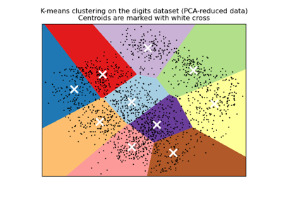
A demo of K-Means clustering on the handwritten digits data

Principal Component Regression vs Partial Least Squares Regression

The Iris Dataset

Blind source separation using FastICA

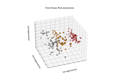
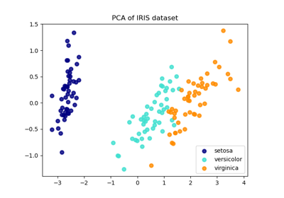
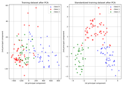
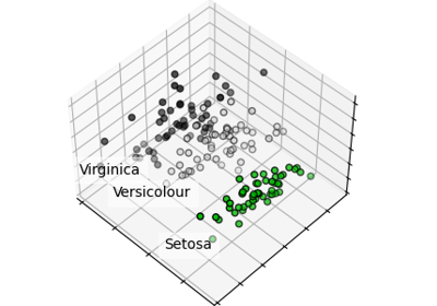
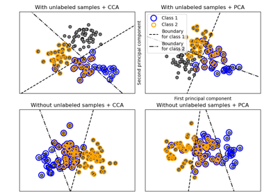
Comparison of LDA and PCA 2D projection of Iris dataset

Faces dataset decompositions

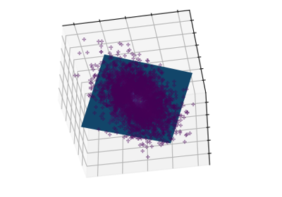
Factor Analysis (with rotation) to visualize patterns

FastICA on 2D point clouds

Incremental PCA

Kernel PCA

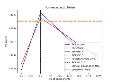
Model selection with Probabilistic PCA and Factor Analysis (FA)

PCA example with Iris Data-set

Principal components analysis (PCA)

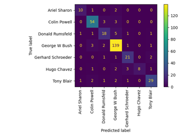
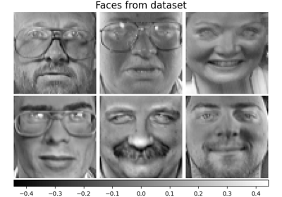
Faces recognition example using eigenfaces and SVMs

Image denoising using kernel PCA

Multi-dimensional scaling

Displaying Pipelines

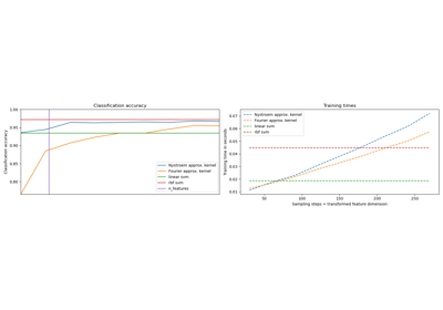
Explicit feature map approximation for RBF kernels

Multilabel classification

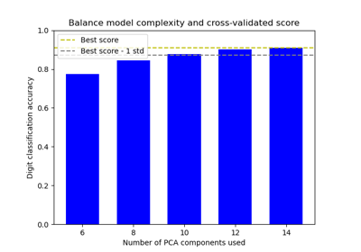
Balance model complexity and cross-validated score

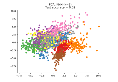
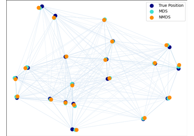
Dimensionality Reduction with Neighborhood Components Analysis

Kernel Density Estimation

Concatenating multiple feature extraction methods

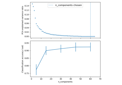
Pipelining: chaining a PCA and a logistic regression

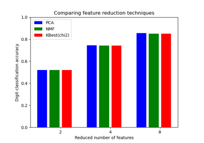
Selecting dimensionality reduction with Pipeline and GridSearchCV

Importance of Feature Scaling

sklearn.decomposition.PCA¶

Examples using sklearn.decomposition.PCA¶

`sklearn.decomposition`.PCA¶

Examples using `sklearn.decomposition.PCA`¶