sklearn.linear_model.SGDClassifier
-
class
sklearn.linear_model.SGDClassifier(loss='hinge', penalty='l2', alpha=0.0001, l1_ratio=0.15, fit_intercept=True, max_iter=1000, tol=0.001, shuffle=True, verbose=0, epsilon=0.1, n_jobs=None, random_state=None, learning_rate='optimal', eta0=0.0, power_t=0.5, early_stopping=False, validation_fraction=0.1, n_iter_no_change=5, class_weight=None, warm_start=False, average=False)[source]¶ Linear classifiers (SVM, logistic regression, a.o.) with SGD training.
This estimator implements regularized linear models with stochastic gradient descent (SGD) learning: the gradient of the loss is estimated each sample at a time and the model is updated along the way with a decreasing strength schedule (aka learning rate). SGD allows minibatch (online/out-of-core) learning, see the partial_fit method. For best results using the default learning rate schedule, the data should have zero mean and unit variance.
This implementation works with data represented as dense or sparse arrays of floating point values for the features. The model it fits can be controlled with the loss parameter; by default, it fits a linear support vector machine (SVM).
The regularizer is a penalty added to the loss function that shrinks model parameters towards the zero vector using either the squared euclidean norm L2 or the absolute norm L1 or a combination of both (Elastic Net). If the parameter update crosses the 0.0 value because of the regularizer, the update is truncated to 0.0 to allow for learning sparse models and achieve online feature selection.
Read more in the User Guide.
- Parameters
- lossstr, default=’hinge’
The loss function to be used. Defaults to ‘hinge’, which gives a linear SVM.
The possible options are ‘hinge’, ‘log’, ‘modified_huber’, ‘squared_hinge’, ‘perceptron’, or a regression loss: ‘squared_loss’, ‘huber’, ‘epsilon_insensitive’, or ‘squared_epsilon_insensitive’.
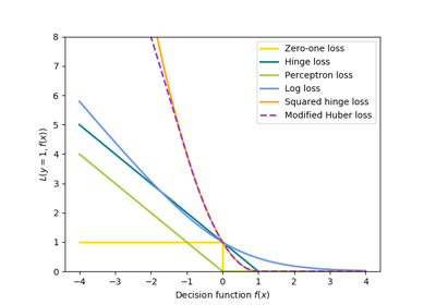
The ‘log’ loss gives logistic regression, a probabilistic classifier. ‘modified_huber’ is another smooth loss that brings tolerance to outliers as well as probability estimates. ‘squared_hinge’ is like hinge but is quadratically penalized. ‘perceptron’ is the linear loss used by the perceptron algorithm. The other losses are designed for regression but can be useful in classification as well; see SGDRegressor for a description.
- penalty{‘l2’, ‘l1’, ‘elasticnet’}, default=’l2’
The penalty (aka regularization term) to be used. Defaults to ‘l2’ which is the standard regularizer for linear SVM models. ‘l1’ and ‘elasticnet’ might bring sparsity to the model (feature selection) not achievable with ‘l2’.
- alphafloat, default=0.0001
Constant that multiplies the regularization term. Defaults to 0.0001. Also used to compute learning_rate when set to ‘optimal’.
- l1_ratiofloat, default=0.15
The Elastic Net mixing parameter, with 0 <= l1_ratio <= 1. l1_ratio=0 corresponds to L2 penalty, l1_ratio=1 to L1. Defaults to 0.15.
- fit_interceptbool, default=True
Whether the intercept should be estimated or not. If False, the data is assumed to be already centered. Defaults to True.
- max_iterint, default=1000
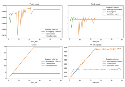
The maximum number of passes over the training data (aka epochs). It only impacts the behavior in the
fitmethod, and not thepartial_fitmethod.New in version 0.19.
- tolfloat, default=1e-3
The stopping criterion. If it is not None, the iterations will stop when (loss > best_loss - tol) for
n_iter_no_changeconsecutive epochs.New in version 0.19.
- shufflebool, default=True
Whether or not the training data should be shuffled after each epoch.
- verboseint, default=0
The verbosity level.
- epsilonfloat, default=0.1
Epsilon in the epsilon-insensitive loss functions; only if
lossis ‘huber’, ‘epsilon_insensitive’, or ‘squared_epsilon_insensitive’. For ‘huber’, determines the threshold at which it becomes less important to get the prediction exactly right. For epsilon-insensitive, any differences between the current prediction and the correct label are ignored if they are less than this threshold.- n_jobsint, default=None
The number of CPUs to use to do the OVA (One Versus All, for multi-class problems) computation.
Nonemeans 1 unless in ajoblib.parallel_backendcontext.-1means using all processors. See Glossary for more details.- random_stateint, RandomState instance, default=None
The seed of the pseudo random number generator to use when shuffling the data. If int, random_state is the seed used by the random number generator; If RandomState instance, random_state is the random number generator; If None, the random number generator is the RandomState instance used by
np.random.- learning_ratestr, default=’optimal’
The learning rate schedule:
- ‘constant’:
eta = eta0
- ‘optimal’: [default]
eta = 1.0 / (alpha * (t + t0)) where t0 is chosen by a heuristic proposed by Leon Bottou.
- ‘invscaling’:
eta = eta0 / pow(t, power_t)
- ‘adaptive’:
eta = eta0, as long as the training keeps decreasing. Each time n_iter_no_change consecutive epochs fail to decrease the training loss by tol or fail to increase validation score by tol if early_stopping is True, the current learning rate is divided by 5.
- eta0double, default=0.0
The initial learning rate for the ‘constant’, ‘invscaling’ or ‘adaptive’ schedules. The default value is 0.0 as eta0 is not used by the default schedule ‘optimal’.
- power_tdouble, default=0.5
The exponent for inverse scaling learning rate [default 0.5].
- early_stoppingbool, default=False
Whether to use early stopping to terminate training when validation score is not improving. If set to True, it will automatically set aside a stratified fraction of training data as validation and terminate training when validation score is not improving by at least tol for n_iter_no_change consecutive epochs.
New in version 0.20.
- validation_fractionfloat, default=0.1
The proportion of training data to set aside as validation set for early stopping. Must be between 0 and 1. Only used if early_stopping is True.
New in version 0.20.
- n_iter_no_changeint, default=5
Number of iterations with no improvement to wait before early stopping.
New in version 0.20.
- class_weightdict, {class_label: weight} or “balanced”, default=None
Preset for the class_weight fit parameter.
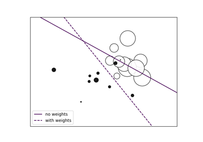
Weights associated with classes. If not given, all classes are supposed to have weight one.
The “balanced” mode uses the values of y to automatically adjust weights inversely proportional to class frequencies in the input data as
n_samples / (n_classes * np.bincount(y)).- warm_startbool, default=False
When set to True, reuse the solution of the previous call to fit as initialization, otherwise, just erase the previous solution. See the Glossary.
Repeatedly calling fit or partial_fit when warm_start is True can result in a different solution than when calling fit a single time because of the way the data is shuffled. If a dynamic learning rate is used, the learning rate is adapted depending on the number of samples already seen. Calling
fitresets this counter, whilepartial_fitwill result in increasing the existing counter.- averagebool or int, default=False
When set to True, computes the averaged SGD weights and stores the result in the
coef_attribute. If set to an int greater than 1, averaging will begin once the total number of samples seen reaches average. Soaverage=10will begin averaging after seeing 10 samples.
- Attributes
- coef_ndarray of shape (1, n_features) if n_classes == 2 else (n_classes, n_features)
Weights assigned to the features.
- intercept_ndarray of shape (1,) if n_classes == 2 else (n_classes,)
Constants in decision function.
- n_iter_int
The actual number of iterations to reach the stopping criterion. For multiclass fits, it is the maximum over every binary fit.
- loss_function_concrete
LossFunction - classes_array of shape (n_classes,)
- t_int
Number of weight updates performed during training. Same as
(n_iter_ * n_samples).
See also
sklearn.svm.LinearSVCLinear support vector classification.
LogisticRegressionLogistic regression.
PerceptronInherits from SGDClassifier.
Perceptron()is equivalent toSGDClassifier(loss="perceptron", eta0=1, learning_rate="constant", penalty=None).
Examples
>>> import numpy as np
>>> from sklearn import linear_model
>>> X = np.array([[-1, -1], [-2, -1], [1, 1], [2, 1]])
>>> Y = np.array([1, 1, 2, 2])
>>> clf = linear_model.SGDClassifier(max_iter=1000, tol=1e-3)
>>> clf.fit(X, Y)
SGDClassifier()
>>> print(clf.predict([[-0.8, -1]]))
[1]
Methods
decision_function(self, X)Predict confidence scores for samples.
densify(self)Convert coefficient matrix to dense array format.
fit(self, X, y[, coef_init, intercept_init, …])Fit linear model with Stochastic Gradient Descent.
get_params(self[, deep])Get parameters for this estimator.
partial_fit(self, X, y[, classes, sample_weight])Perform one epoch of stochastic gradient descent on given samples.
predict(self, X)Predict class labels for samples in X.
score(self, X, y[, sample_weight])Return the mean accuracy on the given test data and labels.
set_params(self, \*\*kwargs)Set and validate the parameters of estimator.
sparsify(self)Convert coefficient matrix to sparse format.
-
__init__(self, loss='hinge', penalty='l2', alpha=0.0001, l1_ratio=0.15, fit_intercept=True, max_iter=1000, tol=0.001, shuffle=True, verbose=0, epsilon=0.1, n_jobs=None, random_state=None, learning_rate='optimal', eta0=0.0, power_t=0.5, early_stopping=False, validation_fraction=0.1, n_iter_no_change=5, class_weight=None, warm_start=False, average=False)[source]¶ Initialize self. See help(type(self)) for accurate signature.
-
decision_function(self, X)[source]¶ Predict confidence scores for samples.
The confidence score for a sample is the signed distance of that sample to the hyperplane.
- Parameters
- Xarray_like or sparse matrix, shape (n_samples, n_features)
Samples.
- Returns
- array, shape=(n_samples,) if n_classes == 2 else (n_samples, n_classes)
Confidence scores per (sample, class) combination. In the binary case, confidence score for self.classes_[1] where >0 means this class would be predicted.
-
densify(self)[source]¶ Convert coefficient matrix to dense array format.
Converts the
coef_member (back) to a numpy.ndarray. This is the default format ofcoef_and is required for fitting, so calling this method is only required on models that have previously been sparsified; otherwise, it is a no-op.- Returns
- self
Fitted estimator.
-
fit(self, X, y, coef_init=None, intercept_init=None, sample_weight=None)[source]¶ Fit linear model with Stochastic Gradient Descent.
- Parameters
- X{array-like, sparse matrix}, shape (n_samples, n_features)
Training data.
- yndarray of shape (n_samples,)
Target values.
- coef_initndarray of shape (n_classes, n_features), default=None
The initial coefficients to warm-start the optimization.
- intercept_initndarray of shape (n_classes,), default=None
The initial intercept to warm-start the optimization.
- sample_weightarray-like, shape (n_samples,), default=None
Weights applied to individual samples. If not provided, uniform weights are assumed. These weights will be multiplied with class_weight (passed through the constructor) if class_weight is specified.
- Returns
- self :
Returns an instance of self.
-
get_params(self, deep=True)[source]¶ Get parameters for this estimator.
- Parameters
- deepbool, default=True
If True, will return the parameters for this estimator and contained subobjects that are estimators.
- Returns
- paramsmapping of string to any
Parameter names mapped to their values.
-
partial_fit(self, X, y, classes=None, sample_weight=None)[source]¶ Perform one epoch of stochastic gradient descent on given samples.
Internally, this method uses
max_iter = 1. Therefore, it is not guaranteed that a minimum of the cost function is reached after calling it once. Matters such as objective convergence and early stopping should be handled by the user.- Parameters
- X{array-like, sparse matrix}, shape (n_samples, n_features)
Subset of the training data.
- yndarray of shape (n_samples,)
Subset of the target values.
- classesndarray of shape (n_classes,), default=None
Classes across all calls to partial_fit. Can be obtained by via
np.unique(y_all), where y_all is the target vector of the entire dataset. This argument is required for the first call to partial_fit and can be omitted in the subsequent calls. Note that y doesn’t need to contain all labels inclasses.- sample_weightarray-like, shape (n_samples,), default=None
Weights applied to individual samples. If not provided, uniform weights are assumed.
- Returns
- self :
Returns an instance of self.
-
predict(self, X)[source]¶ Predict class labels for samples in X.
- Parameters
- Xarray_like or sparse matrix, shape (n_samples, n_features)
Samples.
- Returns
- Carray, shape [n_samples]
Predicted class label per sample.
-
property
predict_log_proba¶ Log of probability estimates.
This method is only available for log loss and modified Huber loss.
When loss=”modified_huber”, probability estimates may be hard zeros and ones, so taking the logarithm is not possible.
See
predict_probafor details.- Parameters
- X{array-like, sparse matrix} of shape (n_samples, n_features)
Input data for prediction.
- Returns
- Tarray-like, shape (n_samples, n_classes)
Returns the log-probability of the sample for each class in the model, where classes are ordered as they are in
self.classes_.
-
property
predict_proba¶ Probability estimates.
This method is only available for log loss and modified Huber loss.
Multiclass probability estimates are derived from binary (one-vs.-rest) estimates by simple normalization, as recommended by Zadrozny and Elkan.
Binary probability estimates for loss=”modified_huber” are given by (clip(decision_function(X), -1, 1) + 1) / 2. For other loss functions it is necessary to perform proper probability calibration by wrapping the classifier with
sklearn.calibration.CalibratedClassifierCVinstead.- Parameters
- X{array-like, sparse matrix}, shape (n_samples, n_features)
Input data for prediction.
- Returns
- ndarray of shape (n_samples, n_classes)
Returns the probability of the sample for each class in the model, where classes are ordered as they are in
self.classes_.
References
Zadrozny and Elkan, “Transforming classifier scores into multiclass probability estimates”, SIGKDD’02, http://www.research.ibm.com/people/z/zadrozny/kdd2002-Transf.pdf
The justification for the formula in the loss=”modified_huber” case is in the appendix B in: http://jmlr.csail.mit.edu/papers/volume2/zhang02c/zhang02c.pdf
-
score(self, X, y, sample_weight=None)[source]¶ Return the mean accuracy on the given test data and labels.
In multi-label classification, this is the subset accuracy which is a harsh metric since you require for each sample that each label set be correctly predicted.
- Parameters
- Xarray-like of shape (n_samples, n_features)
Test samples.
- yarray-like of shape (n_samples,) or (n_samples, n_outputs)
True labels for X.
- sample_weightarray-like of shape (n_samples,), default=None
Sample weights.
- Returns
- scorefloat
Mean accuracy of self.predict(X) wrt. y.
-
set_params(self, **kwargs)[source]¶ Set and validate the parameters of estimator.
- Parameters
- **kwargsdict
Estimator parameters.
- Returns
- selfobject
Estimator instance.
-
sparsify(self)[source]¶ Convert coefficient matrix to sparse format.
Converts the
coef_member to a scipy.sparse matrix, which for L1-regularized models can be much more memory- and storage-efficient than the usual numpy.ndarray representation.The
intercept_member is not converted.- Returns
- self
Fitted estimator.
Notes
For non-sparse models, i.e. when there are not many zeros in
coef_, this may actually increase memory usage, so use this method with care. A rule of thumb is that the number of zero elements, which can be computed with(coef_ == 0).sum(), must be more than 50% for this to provide significant benefits.After calling this method, further fitting with the partial_fit method (if any) will not work until you call densify.

