1.11. Ensemble methods

The goal of ensemble methods is to combine the predictions of several base estimators built with a given learning algorithm in order to improve generalizability / robustness over a single estimator.

Two families of ensemble methods are usually distinguished:

• In averaging methods, the driving principle is to build several estimators independently and then to average their predictions. On average, the combined estimator is usually better than any of the single base estimator because its variance is reduced.

  Examples: Bagging methods, Forests of randomized trees, …

• By contrast, in boosting methods, base estimators are built sequentially and one tries to reduce the bias of the combined estimator. The motivation is to combine several weak models to produce a powerful ensemble.

  Examples: AdaBoost, Gradient Tree Boosting, …

1.11.1. Bagging meta-estimator

In ensemble algorithms, bagging methods form a class of algorithms which build several instances of a black-box estimator on random subsets of the original training set and then aggregate their individual predictions to form a final prediction. These methods are used as a way to reduce the variance of a base estimator (e.g., a decision tree), by introducing randomization into its construction procedure and then making an ensemble out of it. In many cases, bagging methods constitute a very simple way to improve with respect to a single model, without making it necessary to adapt the underlying base algorithm. As they provide a way to reduce overfitting, bagging methods work best with strong and complex models (e.g., fully developed decision trees), in contrast with boosting methods which usually work best with weak models (e.g., shallow decision trees).

Bagging methods come in many flavours but mostly differ from each other by the way they draw random subsets of the training set:

• When random subsets of the dataset are drawn as random subsets of the samples, then this algorithm is known as Pasting [B1999].
• When samples are drawn with replacement, then the method is known as Bagging [B1996].
• When random subsets of the dataset are drawn as random subsets of the features, then the method is known as Random Subspaces [H1998].
• Finally, when base estimators are built on subsets of both samples and features, then the method is known as Random Patches [LG2012].

In scikit-learn, bagging methods are offered as a unified BaggingClassifier meta-estimator (resp. BaggingRegressor), taking as input a user-specified base estimator along with parameters specifying the strategy to draw random subsets. In particular, max_samples and max_features control the size of the subsets (in terms of samples and features), while bootstrap and bootstrap_features control whether samples and features are drawn with or without replacement. When using a subset of the available samples the generalization accuracy can be estimated with the out-of-bag samples by setting oob_score=True. As an example, the snippet below illustrates how to instantiate a bagging ensemble of KNeighborsClassifier base estimators, each built on random subsets of 50% of the samples and 50% of the features.

>>> from sklearn.ensemble import BaggingClassifier
>>> from sklearn.neighbors import KNeighborsClassifier
>>> bagging = BaggingClassifier(KNeighborsClassifier(),
...                             max_samples=0.5, max_features=0.5)

Examples:

• Single estimator versus bagging: bias-variance decomposition

References

[B1999]

L. Breiman, “Pasting small votes for classification in large databases and on-line”, Machine Learning, 36(1), 85-103, 1999.

[B1996]

L. Breiman, “Bagging predictors”, Machine Learning, 24(2), 123-140, 1996.

[H1998]

T. Ho, “The random subspace method for constructing decision forests”, Pattern Analysis and Machine Intelligence, 20(8), 832-844, 1998.

[LG2012]

G. Louppe and P. Geurts, “Ensembles on Random Patches”, Machine Learning and Knowledge Discovery in Databases, 346-361, 2012.

1.11.2. Forests of randomized trees

The sklearn.ensemble module includes two averaging algorithms based on randomized decision trees: the RandomForest algorithm and the Extra-Trees method. Both algorithms are perturb-and-combine techniques [B1998] specifically designed for trees. This means a diverse set of classifiers is created by introducing randomness in the classifier construction. The prediction of the ensemble is given as the averaged prediction of the individual classifiers.

As other classifiers, forest classifiers have to be fitted with two arrays: a sparse or dense array X of size [n_samples, n_features] holding the training samples, and an array Y of size [n_samples] holding the target values (class labels) for the training samples:

>>> from sklearn.ensemble import RandomForestClassifier
>>> X = [[0, 0], [1, 1]]
>>> Y = [0, 1]
>>> clf = RandomForestClassifier(n_estimators=10)
>>> clf = clf.fit(X, Y)

Like decision trees, forests of trees also extend to multi-output problems (if Y is an array of size [n_samples, n_outputs]).

1.11.2.1. Random Forests

In random forests (see RandomForestClassifier and RandomForestRegressor classes), each tree in the ensemble is built from a sample drawn with replacement (i.e., a bootstrap sample) from the training set.

Furthermore, when splitting each node during the construction of a tree, the best split is found either from all input features or a random subset of size max_features. (See the parameter tuning guidelines for more details).

The purpose of these two sources of randomness is to decrease the variance of the forest estimator. Indeed, individual decision trees typically exhibit high variance and tend to overfit. The injected randomness in forests yield decision trees with somewhat decoupled prediction errors. By taking an average of those predictions, some errors can cancel out. Random forests achieve a reduced variance by combining diverse trees, sometimes at the cost of a slight increase in bias. In practice the variance reduction is often significant hence yielding an overall better model.

In contrast to the original publication [B2001], the scikit-learn implementation combines classifiers by averaging their probabilistic prediction, instead of letting each classifier vote for a single class.

1.11.2.2. Extremely Randomized Trees

In extremely randomized trees (see ExtraTreesClassifier and ExtraTreesRegressor classes), randomness goes one step further in the way splits are computed. As in random forests, a random subset of candidate features is used, but instead of looking for the most discriminative thresholds, thresholds are drawn at random for each candidate feature and the best of these randomly-generated thresholds is picked as the splitting rule. This usually allows to reduce the variance of the model a bit more, at the expense of a slightly greater increase in bias:

>>> from sklearn.model_selection import cross_val_score
>>> from sklearn.datasets import make_blobs
>>> from sklearn.ensemble import RandomForestClassifier
>>> from sklearn.ensemble import ExtraTreesClassifier
>>> from sklearn.tree import DecisionTreeClassifier

>>> X, y = make_blobs(n_samples=10000, n_features=10, centers=100,
...     random_state=0)

>>> clf = DecisionTreeClassifier(max_depth=None, min_samples_split=2,
...     random_state=0)
>>> scores = cross_val_score(clf, X, y, cv=5)
>>> scores.mean()                               
0.98...

>>> clf = RandomForestClassifier(n_estimators=10, max_depth=None,
...     min_samples_split=2, random_state=0)
>>> scores = cross_val_score(clf, X, y, cv=5)
>>> scores.mean()                               
0.999...

>>> clf = ExtraTreesClassifier(n_estimators=10, max_depth=None,
...     min_samples_split=2, random_state=0)
>>> scores = cross_val_score(clf, X, y, cv=5)
>>> scores.mean() > 0.999
True

1.11.2.3. Parameters

The main parameters to adjust when using these methods is n_estimators and max_features. The former is the number of trees in the forest. The larger the better, but also the longer it will take to compute. In addition, note that results will stop getting significantly better beyond a critical number of trees. The latter is the size of the random subsets of features to consider when splitting a node. The lower the greater the reduction of variance, but also the greater the increase in bias. Empirical good default values are max_features=None (always considering all features instead of a random subset) for regression problems, and max_features="sqrt" (using a random subset of size sqrt(n_features)) for classification tasks (where n_features is the number of features in the data). Good results are often achieved when setting max_depth=None in combination with min_samples_split=2 (i.e., when fully developing the trees). Bear in mind though that these values are usually not optimal, and might result in models that consume a lot of RAM. The best parameter values should always be cross-validated. In addition, note that in random forests, bootstrap samples are used by default (bootstrap=True) while the default strategy for extra-trees is to use the whole dataset (bootstrap=False). When using bootstrap sampling the generalization accuracy can be estimated on the left out or out-of-bag samples. This can be enabled by setting oob_score=True.

Note

The size of the model with the default parameters is \(O( M * N * log (N) )\), where \(M\) is the number of trees and \(N\) is the number of samples. In order to reduce the size of the model, you can change these parameters: min_samples_split, max_leaf_nodes, max_depth and min_samples_leaf.

1.11.2.4. Parallelization

Finally, this module also features the parallel construction of the trees and the parallel computation of the predictions through the n_jobs parameter. If n_jobs=k then computations are partitioned into k jobs, and run on k cores of the machine. If n_jobs=-1 then all cores available on the machine are used. Note that because of inter-process communication overhead, the speedup might not be linear (i.e., using k jobs will unfortunately not be k times as fast). Significant speedup can still be achieved though when building a large number of trees, or when building a single tree requires a fair amount of time (e.g., on large datasets).

Examples:

• Plot the decision surfaces of ensembles of trees on the iris dataset
• Pixel importances with a parallel forest of trees
• Face completion with a multi-output estimators

References

[B2001]

Breiman, “Random Forests”, Machine Learning, 45(1), 5-32, 2001.

[B1998]

Breiman, “Arcing Classifiers”, Annals of Statistics 1998.

• P. Geurts, D. Ernst., and L. Wehenkel, “Extremely randomized trees”, Machine Learning, 63(1), 3-42, 2006.

1.11.2.5. Feature importance evaluation

The relative rank (i.e. depth) of a feature used as a decision node in a tree can be used to assess the relative importance of that feature with respect to the predictability of the target variable. Features used at the top of the tree contribute to the final prediction decision of a larger fraction of the input samples. The expected fraction of the samples they contribute to can thus be used as an estimate of the relative importance of the features. In scikit-learn, the fraction of samples a feature contributes to is combined with the decrease in impurity from splitting them to create a normalized estimate of the predictive power of that feature.

By averaging the estimates of predictive ability over several randomized trees one can reduce the variance of such an estimate and use it for feature selection. This is known as the mean decrease in impurity, or MDI. Refer to [L2014] for more information on MDI and feature importance evaluation with Random Forests.

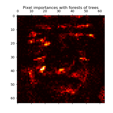
The following example shows a color-coded representation of the relative importances of each individual pixel for a face recognition task using a ExtraTreesClassifier model.

In practice those estimates are stored as an attribute named feature_importances_ on the fitted model. This is an array with shape (n_features,) whose values are positive and sum to 1.0. The higher the value, the more important is the contribution of the matching feature to the prediction function.

Examples:

• Pixel importances with a parallel forest of trees
• Feature importances with forests of trees

References

[L2014]

G. Louppe, “Understanding Random Forests: From Theory to Practice”, PhD Thesis, U. of Liege, 2014.

1.11.2.6. Totally Random Trees Embedding

RandomTreesEmbedding implements an unsupervised transformation of the data. Using a forest of completely random trees, RandomTreesEmbedding encodes the data by the indices of the leaves a data point ends up in. This index is then encoded in a one-of-K manner, leading to a high dimensional, sparse binary coding. This coding can be computed very efficiently and can then be used as a basis for other learning tasks. The size and sparsity of the code can be influenced by choosing the number of trees and the maximum depth per tree. For each tree in the ensemble, the coding contains one entry of one. The size of the coding is at most n_estimators * 2 ** max_depth, the maximum number of leaves in the forest.

As neighboring data points are more likely to lie within the same leaf of a tree, the transformation performs an implicit, non-parametric density estimation.

Examples:

• Hashing feature transformation using Totally Random Trees
• Manifold learning on handwritten digits: Locally Linear Embedding, Isomap… compares non-linear dimensionality reduction techniques on handwritten digits.
• Feature transformations with ensembles of trees compares supervised and unsupervised tree based feature transformations.

See also

Manifold learning techniques can also be useful to derive non-linear representations of feature space, also these approaches focus also on dimensionality reduction.

1.11.3. AdaBoost

The module sklearn.ensemble includes the popular boosting algorithm AdaBoost, introduced in 1995 by Freund and Schapire [FS1995].

The core principle of AdaBoost is to fit a sequence of weak learners (i.e., models that are only slightly better than random guessing, such as small decision trees) on repeatedly modified versions of the data. The predictions from all of them are then combined through a weighted majority vote (or sum) to produce the final prediction. The data modifications at each so-called boosting iteration consist of applying weights \(w_1\), \(w_2\), …, \(w_N\) to each of the training samples. Initially, those weights are all set to \(w_i = 1/N\), so that the first step simply trains a weak learner on the original data. For each successive iteration, the sample weights are individually modified and the learning algorithm is reapplied to the reweighted data. At a given step, those training examples that were incorrectly predicted by the boosted model induced at the previous step have their weights increased, whereas the weights are decreased for those that were predicted correctly. As iterations proceed, examples that are difficult to predict receive ever-increasing influence. Each subsequent weak learner is thereby forced to concentrate on the examples that are missed by the previous ones in the sequence [HTF].

AdaBoost can be used both for classification and regression problems:

• For multi-class classification, AdaBoostClassifier implements AdaBoost-SAMME and AdaBoost-SAMME.R [ZZRH2009].
• For regression, AdaBoostRegressor implements AdaBoost.R2 [D1997].

1.11.3.1. Usage

The following example shows how to fit an AdaBoost classifier with 100 weak learners:

>>> from sklearn.model_selection import cross_val_score
>>> from sklearn.datasets import load_iris
>>> from sklearn.ensemble import AdaBoostClassifier

>>> iris = load_iris()
>>> clf = AdaBoostClassifier(n_estimators=100)
>>> scores = cross_val_score(clf, iris.data, iris.target, cv=5)
>>> scores.mean()                             
0.9...

The number of weak learners is controlled by the parameter n_estimators. The learning_rate parameter controls the contribution of the weak learners in the final combination. By default, weak learners are decision stumps. Different weak learners can be specified through the base_estimator parameter. The main parameters to tune to obtain good results are n_estimators and the complexity of the base estimators (e.g., its depth max_depth or minimum required number of samples to consider a split min_samples_split).

Examples:

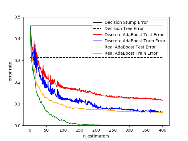
• Discrete versus Real AdaBoost compares the classification error of a decision stump, decision tree, and a boosted decision stump using AdaBoost-SAMME and AdaBoost-SAMME.R.
• Multi-class AdaBoosted Decision Trees shows the performance of AdaBoost-SAMME and AdaBoost-SAMME.R on a multi-class problem.
• Two-class AdaBoost shows the decision boundary and decision function values for a non-linearly separable two-class problem using AdaBoost-SAMME.
• Decision Tree Regression with AdaBoost demonstrates regression with the AdaBoost.R2 algorithm.

References

[FS1995]

Y. Freund, and R. Schapire, “A Decision-Theoretic Generalization of On-Line Learning and an Application to Boosting”, 1997.

[ZZRH2009]

J. Zhu, H. Zou, S. Rosset, T. Hastie. “Multi-class AdaBoost”, 2009.

[D1997]

Drucker. “Improving Regressors using Boosting Techniques”, 1997.

[HTF]

T. Hastie, R. Tibshirani and J. Friedman, “Elements of Statistical Learning Ed. 2”, Springer, 2009.

1.11.4. Gradient Tree Boosting

Gradient Tree Boosting or Gradient Boosted Regression Trees (GBRT) is a generalization of boosting to arbitrary differentiable loss functions. GBRT is an accurate and effective off-the-shelf procedure that can be used for both regression and classification problems. Gradient Tree Boosting models are used in a variety of areas including Web search ranking and ecology.

The advantages of GBRT are:

• Natural handling of data of mixed type (= heterogeneous features)
• Predictive power
• Robustness to outliers in output space (via robust loss functions)

The disadvantages of GBRT are:

• Scalability, due to the sequential nature of boosting it can hardly be parallelized.

The module sklearn.ensemble provides methods for both classification and regression via gradient boosted regression trees.

Note

Scikit-learn 0.21 introduces two new experimental implementation of gradient boosting trees, namely HistGradientBoostingClassifier and HistGradientBoostingRegressor, inspired by LightGBM. These fast estimators first bin the input samples X into integer-valued bins (typically 256 bins) which tremendously reduces the number of splitting points to consider, and allow the algorithm to leverage integer-based data structures (histograms) instead of relying on sorted continuous values.

The new histogram-based estimators can be orders of magnitude faster than their continuous counterparts when the number of samples is larger than tens of thousands of samples. The API of these new estimators is slightly different, and some of the features from GradientBoostingClassifier and GradientBoostingRegressor are not yet supported.

These new estimators are still experimental for now: their predictions and their API might change without any deprecation cycle. To use them, you need to explicitly import enable_hist_gradient_boosting:

>>> # explicitly require this experimental feature
>>> from sklearn.experimental import enable_hist_gradient_boosting  # noqa
>>> # now you can import normally from ensemble
>>> from sklearn.ensemble import HistGradientBoostingClassifier

The following guide focuses on GradientBoostingClassifier and GradientBoostingRegressor only, which might be preferred for small sample sizes since binning may lead to split points that are too approximate in this setting.

1.11.4.1. Classification

GradientBoostingClassifier supports both binary and multi-class classification. The following example shows how to fit a gradient boosting classifier with 100 decision stumps as weak learners:

>>> from sklearn.datasets import make_hastie_10_2
>>> from sklearn.ensemble import GradientBoostingClassifier

>>> X, y = make_hastie_10_2(random_state=0)
>>> X_train, X_test = X[:2000], X[2000:]
>>> y_train, y_test = y[:2000], y[2000:]

>>> clf = GradientBoostingClassifier(n_estimators=100, learning_rate=1.0,
...     max_depth=1, random_state=0).fit(X_train, y_train)
>>> clf.score(X_test, y_test)                 
0.913...

The number of weak learners (i.e. regression trees) is controlled by the parameter n_estimators; The size of each tree can be controlled either by setting the tree depth via max_depth or by setting the number of leaf nodes via max_leaf_nodes. The learning_rate is a hyper-parameter in the range (0.0, 1.0] that controls overfitting via shrinkage .

Note

Classification with more than 2 classes requires the induction of n_classes regression trees at each iteration, thus, the total number of induced trees equals n_classes * n_estimators. For datasets with a large number of classes we strongly recommend to use RandomForestClassifier as an alternative to GradientBoostingClassifier .

1.11.4.2. Regression

GradientBoostingRegressor supports a number of different loss functions for regression which can be specified via the argument loss; the default loss function for regression is least squares ('ls').

>>> import numpy as np
>>> from sklearn.metrics import mean_squared_error
>>> from sklearn.datasets import make_friedman1
>>> from sklearn.ensemble import GradientBoostingRegressor

>>> X, y = make_friedman1(n_samples=1200, random_state=0, noise=1.0)
>>> X_train, X_test = X[:200], X[200:]
>>> y_train, y_test = y[:200], y[200:]
>>> est = GradientBoostingRegressor(n_estimators=100, learning_rate=0.1,
...     max_depth=1, random_state=0, loss='ls').fit(X_train, y_train)
>>> mean_squared_error(y_test, est.predict(X_test))    
5.00...

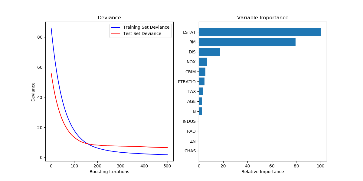
The figure below shows the results of applying GradientBoostingRegressor with least squares loss and 500 base learners to the Boston house price dataset (sklearn.datasets.load_boston). The plot on the left shows the train and test error at each iteration. The train error at each iteration is stored in the train_score_ attribute of the gradient boosting model. The test error at each iterations can be obtained via the staged_predict method which returns a generator that yields the predictions at each stage. Plots like these can be used to determine the optimal number of trees (i.e. n_estimators) by early stopping. The plot on the right shows the feature importances which can be obtained via the feature_importances_ property.

Examples:

• Gradient Boosting regression
• Gradient Boosting Out-of-Bag estimates

1.11.4.3. Fitting additional weak-learners

Both GradientBoostingRegressor and GradientBoostingClassifier support warm_start=True which allows you to add more estimators to an already fitted model.

>>> _ = est.set_params(n_estimators=200, warm_start=True)  # set warm_start and new nr of trees
>>> _ = est.fit(X_train, y_train) # fit additional 100 trees to est
>>> mean_squared_error(y_test, est.predict(X_test))    
3.84...

1.11.4.4. Controlling the tree size

The size of the regression tree base learners defines the level of variable interactions that can be captured by the gradient boosting model. In general, a tree of depth h can capture interactions of order h . There are two ways in which the size of the individual regression trees can be controlled.

If you specify max_depth=h then complete binary trees of depth h will be grown. Such trees will have (at most) 2**h leaf nodes and 2**h - 1 split nodes.

Alternatively, you can control the tree size by specifying the number of leaf nodes via the parameter max_leaf_nodes. In this case, trees will be grown using best-first search where nodes with the highest improvement in impurity will be expanded first. A tree with max_leaf_nodes=k has k - 1 split nodes and thus can model interactions of up to order max_leaf_nodes - 1 .

We found that max_leaf_nodes=k gives comparable results to max_depth=k-1 but is significantly faster to train at the expense of a slightly higher training error. The parameter max_leaf_nodes corresponds to the variable J in the chapter on gradient boosting in [F2001] and is related to the parameter interaction.depth in R’s gbm package where max_leaf_nodes == interaction.depth + 1 .

1.11.4.5. Mathematical formulation

GBRT considers additive models of the following form:

\[F(x) = \sum_{m=1}^{M} \gamma_m h_m(x)\]

where \(h_m(x)\) are the basis functions which are usually called weak learners in the context of boosting. Gradient Tree Boosting uses decision trees of fixed size as weak learners. Decision trees have a number of abilities that make them valuable for boosting, namely the ability to handle data of mixed type and the ability to model complex functions.

Similar to other boosting algorithms, GBRT builds the additive model in a greedy fashion:

\[F_m(x) = F_{m-1}(x) + \gamma_m h_m(x),\]

where the newly added tree \(h_m\) tries to minimize the loss \(L\), given the previous ensemble \(F_{m-1}\):

\[h_m = \arg\min_{h} \sum_{i=1}^{n} L(y_i, F_{m-1}(x_i) + h(x_i)).\]

The initial model \(F_{0}\) is problem specific, for least-squares regression one usually chooses the mean of the target values.

Note

The initial model can also be specified via the init argument. The passed object has to implement fit and predict.

Gradient Boosting attempts to solve this minimization problem numerically via steepest descent: The steepest descent direction is the negative gradient of the loss function evaluated at the current model \(F_{m-1}\) which can be calculated for any differentiable loss function:

\[F_m(x) = F_{m-1}(x) - \gamma_m \sum_{i=1}^{n} \nabla_F L(y_i, F_{m-1}(x_i))\]

Where the step length \(\gamma_m\) is chosen using line search:

\[\gamma_m = \arg\min_{\gamma} \sum_{i=1}^{n} L(y_i, F_{m-1}(x_i) - \gamma \frac{\partial L(y_i, F_{m-1}(x_i))}{\partial F_{m-1}(x_i)})\]

The algorithms for regression and classification only differ in the concrete loss function used.

1.11.4.5.1. Loss Functions

The following loss functions are supported and can be specified using the parameter loss:

• Regression
  • Least squares ('ls'): The natural choice for regression due to its superior computational properties. The initial model is given by the mean of the target values.
  • Least absolute deviation ('lad'): A robust loss function for regression. The initial model is given by the median of the target values.
  • Huber ('huber'): Another robust loss function that combines least squares and least absolute deviation; use alpha to control the sensitivity with regards to outliers (see [F2001] for more details).
  • Quantile ('quantile'): A loss function for quantile regression. Use 0 < alpha < 1 to specify the quantile. This loss function can be used to create prediction intervals (see Prediction Intervals for Gradient Boosting Regression).
• Classification
  • Binomial deviance ('deviance'): The negative binomial log-likelihood loss function for binary classification (provides probability estimates). The initial model is given by the log odds-ratio.
  • Multinomial deviance ('deviance'): The negative multinomial log-likelihood loss function for multi-class classification with n_classes mutually exclusive classes. It provides probability estimates. The initial model is given by the prior probability of each class. At each iteration n_classes regression trees have to be constructed which makes GBRT rather inefficient for data sets with a large number of classes.
  • Exponential loss ('exponential'): The same loss function as AdaBoostClassifier. Less robust to mislabeled examples than 'deviance'; can only be used for binary classification.

1.11.4.6. Regularization

1.11.4.6.1. Shrinkage

[F2001] proposed a simple regularization strategy that scales the contribution of each weak learner by a factor \(\nu\):

\[F_m(x) = F_{m-1}(x) + \nu \gamma_m h_m(x)\]

The parameter \(\nu\) is also called the learning rate because it scales the step length the gradient descent procedure; it can be set via the learning_rate parameter.

The parameter learning_rate strongly interacts with the parameter n_estimators, the number of weak learners to fit. Smaller values of learning_rate require larger numbers of weak learners to maintain a constant training error. Empirical evidence suggests that small values of learning_rate favor better test error. [HTF2009] recommend to set the learning rate to a small constant (e.g. learning_rate <= 0.1) and choose n_estimators by early stopping. For a more detailed discussion of the interaction between learning_rate and n_estimators see [R2007].

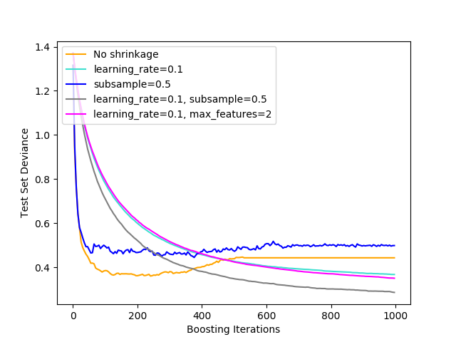
1.11.4.6.2. Subsampling

[F1999] proposed stochastic gradient boosting, which combines gradient boosting with bootstrap averaging (bagging). At each iteration the base classifier is trained on a fraction subsample of the available training data. The subsample is drawn without replacement. A typical value of subsample is 0.5.

The figure below illustrates the effect of shrinkage and subsampling on the goodness-of-fit of the model. We can clearly see that shrinkage outperforms no-shrinkage. Subsampling with shrinkage can further increase the accuracy of the model. Subsampling without shrinkage, on the other hand, does poorly.

Another strategy to reduce the variance is by subsampling the features analogous to the random splits in RandomForestClassifier . The number of subsampled features can be controlled via the max_features parameter.

Note

Using a small max_features value can significantly decrease the runtime.

Stochastic gradient boosting allows to compute out-of-bag estimates of the test deviance by computing the improvement in deviance on the examples that are not included in the bootstrap sample (i.e. the out-of-bag examples). The improvements are stored in the attribute oob_improvement_. oob_improvement_[i] holds the improvement in terms of the loss on the OOB samples if you add the i-th stage to the current predictions. Out-of-bag estimates can be used for model selection, for example to determine the optimal number of iterations. OOB estimates are usually very pessimistic thus we recommend to use cross-validation instead and only use OOB if cross-validation is too time consuming.

Examples:

• Gradient Boosting regularization
• Gradient Boosting Out-of-Bag estimates
• OOB Errors for Random Forests

1.11.4.7. Interpretation

Individual decision trees can be interpreted easily by simply visualizing the tree structure. Gradient boosting models, however, comprise hundreds of regression trees thus they cannot be easily interpreted by visual inspection of the individual trees. Fortunately, a number of techniques have been proposed to summarize and interpret gradient boosting models.

1.11.4.7.1. Feature importance

Often features do not contribute equally to predict the target response; in many situations the majority of the features are in fact irrelevant. When interpreting a model, the first question usually is: what are those important features and how do they contributing in predicting the target response?

Individual decision trees intrinsically perform feature selection by selecting appropriate split points. This information can be used to measure the importance of each feature; the basic idea is: the more often a feature is used in the split points of a tree the more important that feature is. This notion of importance can be extended to decision tree ensembles by simply averaging the feature importance of each tree (see Feature importance evaluation for more details).

The feature importance scores of a fit gradient boosting model can be accessed via the feature_importances_ property:

>>> from sklearn.datasets import make_hastie_10_2
>>> from sklearn.ensemble import GradientBoostingClassifier

>>> X, y = make_hastie_10_2(random_state=0)
>>> clf = GradientBoostingClassifier(n_estimators=100, learning_rate=1.0,
...     max_depth=1, random_state=0).fit(X, y)
>>> clf.feature_importances_  
array([0.10..., 0.10..., 0.11..., ...

Examples:

• Gradient Boosting regression

1.11.5. Voting Classifier

The idea behind the VotingClassifier is to combine conceptually different machine learning classifiers and use a majority vote or the average predicted probabilities (soft vote) to predict the class labels. Such a classifier can be useful for a set of equally well performing model in order to balance out their individual weaknesses.

1.11.5.1. Majority Class Labels (Majority/Hard Voting)

In majority voting, the predicted class label for a particular sample is the class label that represents the majority (mode) of the class labels predicted by each individual classifier.

E.g., if the prediction for a given sample is

• classifier 1 -> class 1
• classifier 2 -> class 1
• classifier 3 -> class 2

the VotingClassifier (with voting='hard') would classify the sample as “class 1” based on the majority class label.

In the cases of a tie, the VotingClassifier will select the class based on the ascending sort order. E.g., in the following scenario

• classifier 1 -> class 2
• classifier 2 -> class 1

the class label 1 will be assigned to the sample.

1.11.5.1.1. Usage

The following example shows how to fit the majority rule classifier:

>>> from sklearn import datasets
>>> from sklearn.model_selection import cross_val_score
>>> from sklearn.linear_model import LogisticRegression
>>> from sklearn.naive_bayes import GaussianNB
>>> from sklearn.ensemble import RandomForestClassifier
>>> from sklearn.ensemble import VotingClassifier

>>> iris = datasets.load_iris()
>>> X, y = iris.data[:, 1:3], iris.target

>>> clf1 = LogisticRegression(solver='lbfgs', multi_class='multinomial',
...                           random_state=1)
>>> clf2 = RandomForestClassifier(n_estimators=50, random_state=1)
>>> clf3 = GaussianNB()

>>> eclf = VotingClassifier(estimators=[('lr', clf1), ('rf', clf2), ('gnb', clf3)], voting='hard')

>>> for clf, label in zip([clf1, clf2, clf3, eclf], ['Logistic Regression', 'Random Forest', 'naive Bayes', 'Ensemble']):
...     scores = cross_val_score(clf, X, y, cv=5, scoring='accuracy')
...     print("Accuracy: %0.2f (+/- %0.2f) [%s]" % (scores.mean(), scores.std(), label))
Accuracy: 0.95 (+/- 0.04) [Logistic Regression]
Accuracy: 0.94 (+/- 0.04) [Random Forest]
Accuracy: 0.91 (+/- 0.04) [naive Bayes]
Accuracy: 0.95 (+/- 0.04) [Ensemble]

1.11.5.2. Weighted Average Probabilities (Soft Voting)

In contrast to majority voting (hard voting), soft voting returns the class label as argmax of the sum of predicted probabilities.

Specific weights can be assigned to each classifier via the weights parameter. When weights are provided, the predicted class probabilities for each classifier are collected, multiplied by the classifier weight, and averaged. The final class label is then derived from the class label with the highest average probability.

To illustrate this with a simple example, let’s assume we have 3 classifiers and a 3-class classification problems where we assign equal weights to all classifiers: w1=1, w2=1, w3=1.

The weighted average probabilities for a sample would then be calculated as follows:

classifier	class 1	class 2	class 3
classifier 1	w1 * 0.2	w1 * 0.5	w1 * 0.3
classifier 2	w2 * 0.6	w2 * 0.3	w2 * 0.1
classifier 3	w3 * 0.3	w3 * 0.4	w3 * 0.3
weighted average	0.37	0.4	0.23

Here, the predicted class label is 2, since it has the highest average probability.

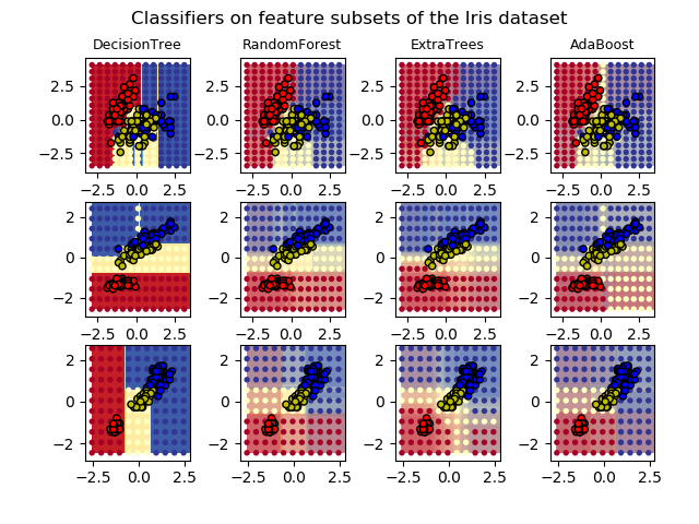
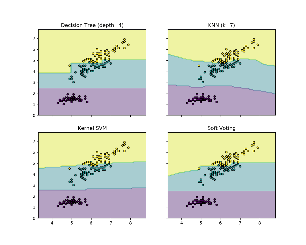
The following example illustrates how the decision regions may change when a soft VotingClassifier is used based on an linear Support Vector Machine, a Decision Tree, and a K-nearest neighbor classifier:

>>> from sklearn import datasets
>>> from sklearn.tree import DecisionTreeClassifier
>>> from sklearn.neighbors import KNeighborsClassifier
>>> from sklearn.svm import SVC
>>> from itertools import product
>>> from sklearn.ensemble import VotingClassifier

>>> # Loading some example data
>>> iris = datasets.load_iris()
>>> X = iris.data[:, [0, 2]]
>>> y = iris.target

>>> # Training classifiers
>>> clf1 = DecisionTreeClassifier(max_depth=4)
>>> clf2 = KNeighborsClassifier(n_neighbors=7)
>>> clf3 = SVC(gamma='scale', kernel='rbf', probability=True)
>>> eclf = VotingClassifier(estimators=[('dt', clf1), ('knn', clf2), ('svc', clf3)],
...                         voting='soft', weights=[2, 1, 2])

>>> clf1 = clf1.fit(X, y)
>>> clf2 = clf2.fit(X, y)
>>> clf3 = clf3.fit(X, y)
>>> eclf = eclf.fit(X, y)

1.11.5.3. Using the VotingClassifier with GridSearchCV

The VotingClassifier can also be used together with GridSearchCV in order to tune the hyperparameters of the individual estimators:

>>> from sklearn.model_selection import GridSearchCV
>>> clf1 = LogisticRegression(solver='lbfgs', multi_class='multinomial',
...                           random_state=1)
>>> clf2 = RandomForestClassifier(random_state=1)
>>> clf3 = GaussianNB()
>>> eclf = VotingClassifier(estimators=[('lr', clf1), ('rf', clf2), ('gnb', clf3)], voting='soft')

>>> params = {'lr__C': [1.0, 100.0], 'rf__n_estimators': [20, 200]}

>>> grid = GridSearchCV(estimator=eclf, param_grid=params, cv=5)
>>> grid = grid.fit(iris.data, iris.target)

1.11.5.3.1. Usage

In order to predict the class labels based on the predicted class-probabilities (scikit-learn estimators in the VotingClassifier must support predict_proba method):

>>> eclf = VotingClassifier(estimators=[('lr', clf1), ('rf', clf2), ('gnb', clf3)], voting='soft')

Optionally, weights can be provided for the individual classifiers:

>>> eclf = VotingClassifier(estimators=[('lr', clf1), ('rf', clf2), ('gnb', clf3)],
...                         voting='soft', weights=[2, 5, 1])

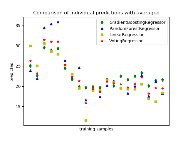
1.11.6. Voting Regressor

The idea behind the VotingRegressor is to combine conceptually different machine learning regressors and return the average predicted values. Such a regressor can be useful for a set of equally well performing models in order to balance out their individual weaknesses.

The following example shows how to fit the VotingRegressor:

>>> from sklearn import datasets
>>> from sklearn.ensemble import GradientBoostingRegressor
>>> from sklearn.ensemble import RandomForestRegressor
>>> from sklearn.linear_model import LinearRegression
>>> from sklearn.ensemble import VotingRegressor

>>> # Loading some example data
>>> boston = datasets.load_boston()
>>> X = boston.data
>>> y = boston.target

>>> # Training classifiers
>>> reg1 = GradientBoostingRegressor(random_state=1, n_estimators=10)
>>> reg2 = RandomForestRegressor(random_state=1, n_estimators=10)
>>> reg3 = LinearRegression()
>>> ereg = VotingRegressor(estimators=[('gb', reg1), ('rf', reg2), ('lr', reg3)])
>>> ereg = ereg.fit(X, y)

Examples:

• Plot individual and voting regression predictions