4.1. Partial dependence plots

Partial dependence plots (PDP) show the dependence between the target response [1] and a set of ‘target’ features, marginalizing over the values of all other features (the ‘complement’ features). Intuitively, we can interpret the partial dependence as the expected target response as a function of the ‘target’ features.

Due to the limits of human perception the size of the target feature set must be small (usually, one or two) thus the target features are usually chosen among the most important features.

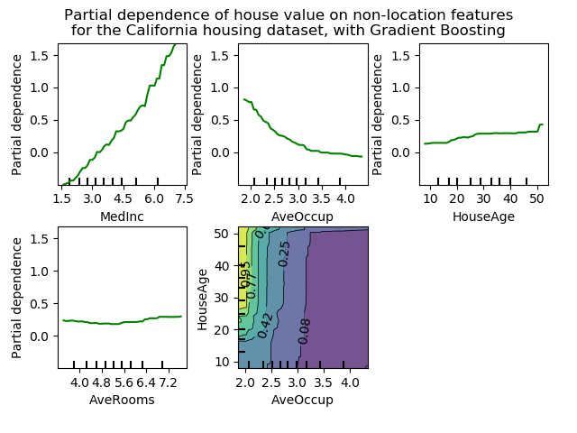
The figure below shows four one-way and one two-way partial dependence plots for the California housing dataset, with a GradientBoostingRegressor:

One-way PDPs tell us about the interaction between the target response and the target feature (e.g. linear, non-linear). The upper left plot in the above figure shows the effect of the median income in a district on the median house price; we can clearly see a linear relationship among them. Note that PDPs assume that the target features are independent from the complement features, and this assumption is often violated in practice.

PDPs with two target features show the interactions among the two features. For example, the two-variable PDP in the above figure shows the dependence of median house price on joint values of house age and average occupants per household. We can clearly see an interaction between the two features: for an average occupancy greater than two, the house price is nearly independent of the house age, whereas for values less than 2 there is a strong dependence on age.

The sklearn.inspection module provides a convenience function plot_partial_dependence to create one-way and two-way partial dependence plots. In the below example we show how to create a grid of partial dependence plots: two one-way PDPs for the features 0 and 1 and a two-way PDP between the two features:

>>> from sklearn.datasets import make_hastie_10_2
>>> from sklearn.ensemble import GradientBoostingClassifier
>>> from sklearn.inspection import plot_partial_dependence

>>> X, y = make_hastie_10_2(random_state=0)
>>> clf = GradientBoostingClassifier(n_estimators=100, learning_rate=1.0,
...     max_depth=1, random_state=0).fit(X, y)
>>> features = [0, 1, (0, 1)]
>>> plot_partial_dependence(clf, X, features) 

You can access the newly created figure and Axes objects using plt.gcf() and plt.gca().

For multi-class classification, you need to set the class label for which the PDPs should be created via the target argument:

>>> from sklearn.datasets import load_iris
>>> iris = load_iris()
>>> mc_clf = GradientBoostingClassifier(n_estimators=10,
...     max_depth=1).fit(iris.data, iris.target)
>>> features = [3, 2, (3, 2)]
>>> plot_partial_dependence(mc_clf, X, features, target=0) 

The same parameter target is used to specify the target in multi-output regression settings.

If you need the raw values of the partial dependence function rather than the plots, you can use the sklearn.inspection.partial_dependence function:

>>> from sklearn.inspection import partial_dependence

>>> pdp, axes = partial_dependence(clf, X, [0])
>>> pdp  
array([[ 2.466...,  2.466..., ...
>>> axes  
[array([-1.624..., -1.592..., ...

The values at which the partial dependence should be evaluated are directly generated from X. For 2-way partial dependence, a 2D-grid of values is generated. The values field returned by sklearn.inspection.partial_dependence gives the actual values used in the grid for each target feature. They also correspond to the axis of the plots.

For each value of the ‘target’ features in the grid the partial dependence function needs to marginalize the predictions of the estimator over all possible values of the ‘complement’ features. With the 'brute' method, this is done by replacing every target feature value of X by those in the grid, and computing the average prediction.

In decision trees this can be evaluated efficiently without reference to the training data ('recursion' method). For each grid point a weighted tree traversal is performed: if a split node involves a ‘target’ feature, the corresponding left or right branch is followed, otherwise both branches are followed, each branch is weighted by the fraction of training samples that entered that branch. Finally, the partial dependence is given by a weighted average of all visited leaves. Note that with the 'recursion' method, X is only used to generate the grid, not to compute the averaged predictions. The averaged predictions will always be computed on the data with which the trees were trained.

Footnotes

[1]	For classification, the target response may be the probability of a class (the positive class for binary classification), or the decision function.

Examples:

• Partial Dependence Plots

References

[HTF2009]

T. Hastie, R. Tibshirani and J. Friedman, The Elements of Statistical Learning, Second Edition, Section 10.13.2, Springer, 2009.

[Mol2019]

C. Molnar, Interpretable Machine Learning, Section 5.1, 2019.