Partial Dependence Plots

Partial dependence plots show the dependence between the target function [2] and a set of ‘target’ features, marginalizing over the values of all other features (the complement features). Due to the limits of human perception the size of the target feature set must be small (usually, one or two) thus the target features are usually chosen among the most important features.

This example shows how to obtain partial dependence plots from a MLPRegressor and a GradientBoostingRegressor trained on the California housing dataset. The example is taken from [1].

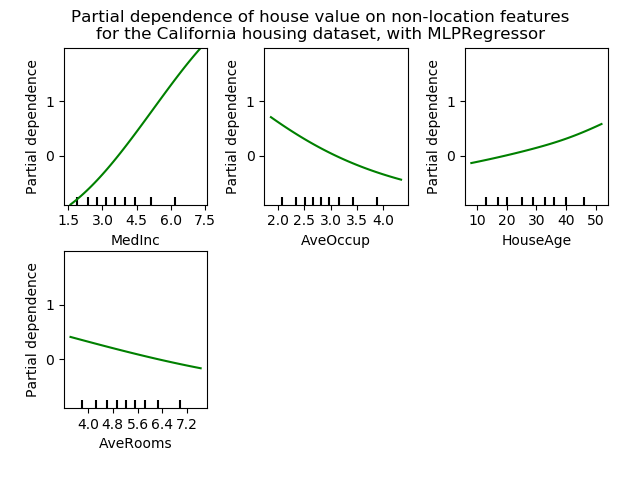
The plots show four 1-way and two 1-way partial dependence plots (ommitted for MLPRegressor due to computation time). The target variables for the one-way PDP are: median income (MedInc), average occupants per household (AvgOccup), median house age (HouseAge), and average rooms per household (AveRooms).

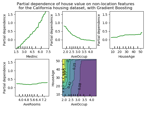
We can clearly see that the median house price shows a linear relationship with the median income (top left) and that the house price drops when the average occupants per household increases (top middle). The top right plot shows that the house age in a district does not have a strong influence on the (median) house price; so does the average rooms per household. The tick marks on the x-axis represent the deciles of the feature values in the training data.

We also observe that MLPRegressor has much smoother predictions than GradientBoostingRegressor. For the plots to be comparable, it is necessary to subtract the average value of the target y: The ‘recursion’ method, used by default for GradientBoostingRegressor, does not account for the initial predictor (in our case the average target). Setting the target average to 0 avoids this bias.

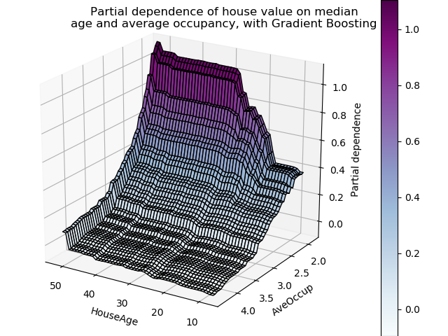
Partial dependence plots with two target features enable us to visualize interactions among them. The two-way partial dependence plot shows the dependence of median house price on joint values of house age and average occupants per household. We can clearly see an interaction between the two features: for an average occupancy greater than two, the house price is nearly independent of the house age, whereas for values less than two there is a strong dependence on age.

On a third figure, we have plotted the same partial dependence plot, this time in 3 dimensions.

[1]	T. Hastie, R. Tibshirani and J. Friedman, “Elements of Statistical Learning Ed. 2”, Springer, 2009.

[2]	For classification you can think of it as the regression score before the link function.

• 
• 
• 

Out:

Training MLPRegressor...
Computing partial dependence plots...
Training GradientBoostingRegressor...
Computing partial dependence plots...
Custom 3d plot via ``partial_dependence``

print(__doc__)

import numpy as np
import matplotlib.pyplot as plt
from mpl_toolkits.mplot3d import Axes3D

from sklearn.inspection import partial_dependence
from sklearn.inspection import plot_partial_dependence
from sklearn.ensemble import GradientBoostingRegressor
from sklearn.neural_network import MLPRegressor
from sklearn.datasets.california_housing import fetch_california_housing


def main():
    cal_housing = fetch_california_housing()

    X, y = cal_housing.data, cal_housing.target
    names = cal_housing.feature_names

    # Center target to avoid gradient boosting init bias: gradient boosting
    # with the 'recursion' method does not account for the initial estimator
    # (here the average target, by default)
    y -= y.mean()

    print("Training MLPRegressor...")
    est = MLPRegressor(activation='logistic')
    est.fit(X, y)
    print('Computing partial dependence plots...')
    # We don't compute the 2-way PDP (5, 1) here, because it is a lot slower
    # with the brute method.
    features = [0, 5, 1, 2]
    plot_partial_dependence(est, X, features, feature_names=names,
                            n_jobs=3, grid_resolution=50)
    fig = plt.gcf()
    fig.suptitle('Partial dependence of house value on non-location features\n'
                 'for the California housing dataset, with MLPRegressor')
    plt.subplots_adjust(top=0.9)  # tight_layout causes overlap with suptitle

    print("Training GradientBoostingRegressor...")
    est = GradientBoostingRegressor(n_estimators=100, max_depth=4,
                                    learning_rate=0.1, loss='huber',
                                    random_state=1)
    est.fit(X, y)
    print('Computing partial dependence plots...')
    features = [0, 5, 1, 2, (5, 1)]
    plot_partial_dependence(est, X, features, feature_names=names,
                            n_jobs=3, grid_resolution=50)
    fig = plt.gcf()
    fig.suptitle('Partial dependence of house value on non-location features\n'
                 'for the California housing dataset, with Gradient Boosting')
    plt.subplots_adjust(top=0.9)

    print('Custom 3d plot via ``partial_dependence``')
    fig = plt.figure()

    target_feature = (1, 5)
    pdp, axes = partial_dependence(est, X, target_feature,
                                   grid_resolution=50)
    XX, YY = np.meshgrid(axes[0], axes[1])
    Z = pdp[0].T
    ax = Axes3D(fig)
    surf = ax.plot_surface(XX, YY, Z, rstride=1, cstride=1,
                           cmap=plt.cm.BuPu, edgecolor='k')
    ax.set_xlabel(names[target_feature[0]])
    ax.set_ylabel(names[target_feature[1]])
    ax.set_zlabel('Partial dependence')
    #  pretty init view
    ax.view_init(elev=22, azim=122)
    plt.colorbar(surf)
    plt.suptitle('Partial dependence of house value on median\n'
                 'age and average occupancy, with Gradient Boosting')
    plt.subplots_adjust(top=0.9)

    plt.show()


# Needed on Windows because plot_partial_dependence uses multiprocessing
if __name__ == '__main__':
    main()

Total running time of the script: ( 0 minutes 24.838 seconds)