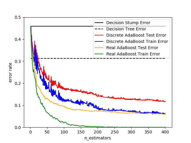
Discrete versus Real AdaBoost

This example is based on Figure 10.2 from Hastie et al 2009 [1] and illustrates the difference in performance between the discrete SAMME [2] boosting algorithm and real SAMME.R boosting algorithm. Both algorithms are evaluated on a binary classification task where the target Y is a non-linear function of 10 input features.

Discrete SAMME AdaBoost adapts based on errors in predicted class labels whereas real SAMME.R uses the predicted class probabilities.

[1]	T. Hastie, R. Tibshirani and J. Friedman, “Elements of Statistical Learning Ed. 2”, Springer, 2009.

[2]	Zhu, H. Zou, S. Rosset, T. Hastie, “Multi-class AdaBoost”, 2009.

print(__doc__)

# Author: Peter Prettenhofer <peter.prettenhofer@gmail.com>,
#         Noel Dawe <noel.dawe@gmail.com>
#
# License: BSD 3 clause

import numpy as np
import matplotlib.pyplot as plt

from sklearn import datasets
from sklearn.tree import DecisionTreeClassifier
from sklearn.metrics import zero_one_loss
from sklearn.ensemble import AdaBoostClassifier


n_estimators = 400
# A learning rate of 1. may not be optimal for both SAMME and SAMME.R
learning_rate = 1.

X, y = datasets.make_hastie_10_2(n_samples=12000, random_state=1)

X_test, y_test = X[2000:], y[2000:]
X_train, y_train = X[:2000], y[:2000]

dt_stump = DecisionTreeClassifier(max_depth=1, min_samples_leaf=1)
dt_stump.fit(X_train, y_train)
dt_stump_err = 1.0 - dt_stump.score(X_test, y_test)

dt = DecisionTreeClassifier(max_depth=9, min_samples_leaf=1)
dt.fit(X_train, y_train)
dt_err = 1.0 - dt.score(X_test, y_test)

ada_discrete = AdaBoostClassifier(
    base_estimator=dt_stump,
    learning_rate=learning_rate,
    n_estimators=n_estimators,
    algorithm="SAMME")
ada_discrete.fit(X_train, y_train)

ada_real = AdaBoostClassifier(
    base_estimator=dt_stump,
    learning_rate=learning_rate,
    n_estimators=n_estimators,
    algorithm="SAMME.R")
ada_real.fit(X_train, y_train)

fig = plt.figure()
ax = fig.add_subplot(111)

ax.plot([1, n_estimators], [dt_stump_err] * 2, 'k-',
        label='Decision Stump Error')
ax.plot([1, n_estimators], [dt_err] * 2, 'k--',
        label='Decision Tree Error')

ada_discrete_err = np.zeros((n_estimators,))
for i, y_pred in enumerate(ada_discrete.staged_predict(X_test)):
    ada_discrete_err[i] = zero_one_loss(y_pred, y_test)

ada_discrete_err_train = np.zeros((n_estimators,))
for i, y_pred in enumerate(ada_discrete.staged_predict(X_train)):
    ada_discrete_err_train[i] = zero_one_loss(y_pred, y_train)

ada_real_err = np.zeros((n_estimators,))
for i, y_pred in enumerate(ada_real.staged_predict(X_test)):
    ada_real_err[i] = zero_one_loss(y_pred, y_test)

ada_real_err_train = np.zeros((n_estimators,))
for i, y_pred in enumerate(ada_real.staged_predict(X_train)):
    ada_real_err_train[i] = zero_one_loss(y_pred, y_train)

ax.plot(np.arange(n_estimators) + 1, ada_discrete_err,
        label='Discrete AdaBoost Test Error',
        color='red')
ax.plot(np.arange(n_estimators) + 1, ada_discrete_err_train,
        label='Discrete AdaBoost Train Error',
        color='blue')
ax.plot(np.arange(n_estimators) + 1, ada_real_err,
        label='Real AdaBoost Test Error',
        color='orange')
ax.plot(np.arange(n_estimators) + 1, ada_real_err_train,
        label='Real AdaBoost Train Error',
        color='green')

ax.set_ylim((0.0, 0.5))
ax.set_xlabel('n_estimators')
ax.set_ylabel('error rate')

leg = ax.legend(loc='upper right', fancybox=True)
leg.get_frame().set_alpha(0.7)

plt.show()

Total running time of the script: ( 0 minutes 4.579 seconds)