5. Dataset loading utilities

The sklearn.datasets package embeds some small toy datasets as introduced in the Getting Started section.

This package also features helpers to fetch larger datasets commonly used by the machine learning community to benchmark algorithms on data that comes from the ‘real world’.

To evaluate the impact of the scale of the dataset (n_samples and n_features) while controlling the statistical properties of the data (typically the correlation and informativeness of the features), it is also possible to generate synthetic data.

5.1. General dataset API

There are three main kinds of dataset interfaces that can be used to get datasets depending on the desired type of dataset.

The dataset loaders. They can be used to load small standard datasets, described in the Toy datasets section.

The dataset fetchers. They can be used to download and load larger datasets, described in the Real world datasets section.

Both loaders and fetchers functions return a dictionary-like object holding at least two items: an array of shape n_samples * n_features with key data (except for 20newsgroups) and a numpy array of length n_samples, containing the target values, with key target.

It’s also possible for almost all of these function to constrain the output to be a tuple containing only the data and the target, by setting the return_X_y parameter to True.

The datasets also contain a full description in their DESCR attribute and some contain feature_names and target_names. See the dataset descriptions below for details.

The dataset generation functions. They can be used to generate controlled synthetic datasets, described in the Generated datasets section.

These functions return a tuple (X, y) consisting of a n_samples * n_features numpy array X and an array of length n_samples containing the targets y.

In addition, there are also miscellanous tools to load datasets of other formats or from other locations, described in the Loading other datasets section.

5.2. Toy datasets

scikit-learn comes with a few small standard datasets that do not require to download any file from some external website.

They can be loaded using the following functions:

load_boston([return_X_y])	Load and return the boston house-prices dataset (regression).
load_iris([return_X_y])	Load and return the iris dataset (classification).
load_diabetes([return_X_y])	Load and return the diabetes dataset (regression).
load_digits([n_class, return_X_y])	Load and return the digits dataset (classification).
load_linnerud([return_X_y])	Load and return the linnerud dataset (multivariate regression).
load_wine([return_X_y])	Load and return the wine dataset (classification).
load_breast_cancer([return_X_y])	Load and return the breast cancer wisconsin dataset (classification).

These datasets are useful to quickly illustrate the behavior of the various algorithms implemented in scikit-learn. They are however often too small to be representative of real world machine learning tasks.

5.2.1. Boston house prices dataset

Data Set Characteristics:

Number of Instances:  

506

Number of Attributes:  

13 numeric/categorical predictive. Median Value (attribute 14) is usually the target.

Attribute Information (in order):  

• CRIM per capita crime rate by town
• ZN proportion of residential land zoned for lots over 25,000 sq.ft.
• INDUS proportion of non-retail business acres per town
• CHAS Charles River dummy variable (= 1 if tract bounds river; 0 otherwise)
• NOX nitric oxides concentration (parts per 10 million)
• RM average number of rooms per dwelling
• AGE proportion of owner-occupied units built prior to 1940
• DIS weighted distances to five Boston employment centres
• RAD index of accessibility to radial highways
• TAX full-value property-tax rate per $10,000
• PTRATIO pupil-teacher ratio by town
• B 1000(Bk - 0.63)^2 where Bk is the proportion of blacks by town
• LSTAT % lower status of the population
• MEDV Median value of owner-occupied homes in $1000’s

Missing Attribute Values:  

None

Creator:

Harrison, D. and Rubinfeld, D.L.

This is a copy of UCI ML housing dataset. https://archive.ics.uci.edu/ml/machine-learning-databases/housing/

This dataset was taken from the StatLib library which is maintained at Carnegie Mellon University.

The Boston house-price data of Harrison, D. and Rubinfeld, D.L. ‘Hedonic prices and the demand for clean air’, J. Environ. Economics & Management, vol.5, 81-102, 1978. Used in Belsley, Kuh & Welsch, ‘Regression diagnostics …’, Wiley, 1980. N.B. Various transformations are used in the table on pages 244-261 of the latter.

The Boston house-price data has been used in many machine learning papers that address regression problems.

References

• Belsley, Kuh & Welsch, ‘Regression diagnostics: Identifying Influential Data and Sources of Collinearity’, Wiley, 1980. 244-261.
• Quinlan,R. (1993). Combining Instance-Based and Model-Based Learning. In Proceedings on the Tenth International Conference of Machine Learning, 236-243, University of Massachusetts, Amherst. Morgan Kaufmann.

5.2.2. Iris plants dataset

Data Set Characteristics:

Number of Instances:  

150 (50 in each of three classes)

Number of Attributes:  

4 numeric, predictive attributes and the class

Attribute Information:  

• sepal length in cm
• sepal width in cm
• petal length in cm
• petal width in cm

• class:

  • Iris-Setosa
  • Iris-Versicolour
  • Iris-Virginica

Summary Statistics:  

sepal length:	4.3	7.9	5.84	0.83	0.7826
sepal width:	2.0	4.4	3.05	0.43	-0.4194
petal length:	1.0	6.9	3.76	1.76	0.9490 (high!)
petal width:	0.1	2.5	1.20	0.76	0.9565 (high!)

Missing Attribute Values:  None Class Distribution:  33.3% for each of 3 classes. Creator:R.A. Fisher Donor:Michael Marshall (MARSHALL%PLU@io.arc.nasa.gov) Date:July, 1988

The famous Iris database, first used by Sir R.A. Fisher. The dataset is taken from Fisher’s paper. Note that it’s the same as in R, but not as in the UCI Machine Learning Repository, which has two wrong data points.

This is perhaps the best known database to be found in the pattern recognition literature. Fisher’s paper is a classic in the field and is referenced frequently to this day. (See Duda & Hart, for example.) The data set contains 3 classes of 50 instances each, where each class refers to a type of iris plant. One class is linearly separable from the other 2; the latter are NOT linearly separable from each other.

References

• Fisher, R.A. “The use of multiple measurements in taxonomic problems” Annual Eugenics, 7, Part II, 179-188 (1936); also in “Contributions to Mathematical Statistics” (John Wiley, NY, 1950).
• Duda, R.O., & Hart, P.E. (1973) Pattern Classification and Scene Analysis. (Q327.D83) John Wiley & Sons. ISBN 0-471-22361-1. See page 218.
• Dasarathy, B.V. (1980) “Nosing Around the Neighborhood: A New System Structure and Classification Rule for Recognition in Partially Exposed Environments”. IEEE Transactions on Pattern Analysis and Machine Intelligence, Vol. PAMI-2, No. 1, 67-71.
• Gates, G.W. (1972) “The Reduced Nearest Neighbor Rule”. IEEE Transactions on Information Theory, May 1972, 431-433.
• See also: 1988 MLC Proceedings, 54-64. Cheeseman et al”s AUTOCLASS II conceptual clustering system finds 3 classes in the data.
• Many, many more …

5.2.3. Diabetes dataset

Ten baseline variables, age, sex, body mass index, average blood pressure, and six blood serum measurements were obtained for each of n = 442 diabetes patients, as well as the response of interest, a quantitative measure of disease progression one year after baseline.

Data Set Characteristics:

Number of Instances:  

442

Number of Attributes:  

First 10 columns are numeric predictive values

Target:

Column 11 is a quantitative measure of disease progression one year after baseline

Attribute Information:  

• Age
• Sex
• Body mass index
• Average blood pressure
• S1
• S2
• S3
• S4
• S5
• S6

Note: Each of these 10 feature variables have been mean centered and scaled by the standard deviation times n_samples (i.e. the sum of squares of each column totals 1).

Source URL: http://www4.stat.ncsu.edu/~boos/var.select/diabetes.html

For more information see: Bradley Efron, Trevor Hastie, Iain Johnstone and Robert Tibshirani (2004) “Least Angle Regression,” Annals of Statistics (with discussion), 407-499. (http://web.stanford.edu/~hastie/Papers/LARS/LeastAngle_2002.pdf)

5.2.4. Optical recognition of handwritten digits dataset

Data Set Characteristics:

Number of Instances:  

5620

Number of Attributes:  

64

Attribute Information:  

8x8 image of integer pixels in the range 0..16.

Missing Attribute Values:  

None

Creator:

5. Alpaydin (alpaydin ‘@’ boun.edu.tr)

Date:

July; 1998

This is a copy of the test set of the UCI ML hand-written digits datasets http://archive.ics.uci.edu/ml/datasets/Optical+Recognition+of+Handwritten+Digits

The data set contains images of hand-written digits: 10 classes where each class refers to a digit.

Preprocessing programs made available by NIST were used to extract normalized bitmaps of handwritten digits from a preprinted form. From a total of 43 people, 30 contributed to the training set and different 13 to the test set. 32x32 bitmaps are divided into nonoverlapping blocks of 4x4 and the number of on pixels are counted in each block. This generates an input matrix of 8x8 where each element is an integer in the range 0..16. This reduces dimensionality and gives invariance to small distortions.

For info on NIST preprocessing routines, see M. D. Garris, J. L. Blue, G. T. Candela, D. L. Dimmick, J. Geist, P. J. Grother, S. A. Janet, and C. L. Wilson, NIST Form-Based Handprint Recognition System, NISTIR 5469, 1994.

References

• C. Kaynak (1995) Methods of Combining Multiple Classifiers and Their Applications to Handwritten Digit Recognition, MSc Thesis, Institute of Graduate Studies in Science and Engineering, Bogazici University.
• 5. Alpaydin, C. Kaynak (1998) Cascading Classifiers, Kybernetika.
• Ken Tang and Ponnuthurai N. Suganthan and Xi Yao and A. Kai Qin. Linear dimensionalityreduction using relevance weighted LDA. School of Electrical and Electronic Engineering Nanyang Technological University. 2005.
• Claudio Gentile. A New Approximate Maximal Margin Classification Algorithm. NIPS. 2000.

5.2.5. Linnerrud dataset

Data Set Characteristics:

Number of Instances:  20 Number of Attributes:  3 Missing Attribute Values:  None

The Linnerud dataset constains two small dataset:

• physiological - CSV containing 20 observations on 3 exercise variables:

  Weight, Waist and Pulse.

• exercise - CSV containing 20 observations on 3 physiological variables:

  Chins, Situps and Jumps.

References

• Tenenhaus, M. (1998). La regression PLS: theorie et pratique. Paris: Editions Technic.

5.2.6. Wine recognition dataset

Data Set Characteristics:

Number of Instances:  

178 (50 in each of three classes)

Number of Attributes:  

13 numeric, predictive attributes and the class

Attribute Information:  

• Alcohol
• Malic acid
• Ash
• Alcalinity of ash
• Magnesium
• Total phenols
• Flavanoids
• Nonflavanoid phenols
• Proanthocyanins
• Color intensity
• Hue
• OD280/OD315 of diluted wines
• Proline

• class:

  • class_0
  • class_1
  • class_2

Summary Statistics:  

Alcohol:	11.0	14.8	13.0	0.8
Malic Acid:	0.74	5.80	2.34	1.12
Ash:	1.36	3.23	2.36	0.27
Alcalinity of Ash:	10.6	30.0	19.5	3.3
Magnesium:	70.0	162.0	99.7	14.3
Total Phenols:	0.98	3.88	2.29	0.63
Flavanoids:	0.34	5.08	2.03	1.00
Nonflavanoid Phenols:	0.13	0.66	0.36	0.12
Proanthocyanins:	0.41	3.58	1.59	0.57
Colour Intensity:	1.3	13.0	5.1	2.3
Hue:	0.48	1.71	0.96	0.23
OD280/OD315 of diluted wines:	1.27	4.00	2.61	0.71
Proline:	278	1680	746	315

Missing Attribute Values:  None Class Distribution:  class_0 (59), class_1 (71), class_2 (48) Creator:R.A. Fisher Donor:Michael Marshall (MARSHALL%PLU@io.arc.nasa.gov) Date:July, 1988

This is a copy of UCI ML Wine recognition datasets. https://archive.ics.uci.edu/ml/machine-learning-databases/wine/wine.data

The data is the results of a chemical analysis of wines grown in the same region in Italy by three different cultivators. There are thirteen different measurements taken for different constituents found in the three types of wine.

Original Owners:

Forina, M. et al, PARVUS - An Extendible Package for Data Exploration, Classification and Correlation. Institute of Pharmaceutical and Food Analysis and Technologies, Via Brigata Salerno, 16147 Genoa, Italy.

Citation:

Lichman, M. (2013). UCI Machine Learning Repository [http://archive.ics.uci.edu/ml]. Irvine, CA: University of California, School of Information and Computer Science.

References

(1) S. Aeberhard, D. Coomans and O. de Vel, Comparison of Classifiers in High Dimensional Settings, Tech. Rep. no. 92-02, (1992), Dept. of Computer Science and Dept. of Mathematics and Statistics, James Cook University of North Queensland. (Also submitted to Technometrics).

The data was used with many others for comparing various classifiers. The classes are separable, though only RDA has achieved 100% correct classification. (RDA : 100%, QDA 99.4%, LDA 98.9%, 1NN 96.1% (z-transformed data)) (All results using the leave-one-out technique)

(2) S. Aeberhard, D. Coomans and O. de Vel, “THE CLASSIFICATION PERFORMANCE OF RDA” Tech. Rep. no. 92-01, (1992), Dept. of Computer Science and Dept. of Mathematics and Statistics, James Cook University of North Queensland. (Also submitted to Journal of Chemometrics).

5.2.7. Breast cancer wisconsin (diagnostic) dataset

Data Set Characteristics:

Number of Instances:  

569

Number of Attributes:  

30 numeric, predictive attributes and the class

Attribute Information:  

• radius (mean of distances from center to points on the perimeter)
• texture (standard deviation of gray-scale values)
• perimeter
• area
• smoothness (local variation in radius lengths)
• compactness (perimeter^2 / area - 1.0)
• concavity (severity of concave portions of the contour)
• concave points (number of concave portions of the contour)
• symmetry
• fractal dimension (“coastline approximation” - 1)

The mean, standard error, and “worst” or largest (mean of the three largest values) of these features were computed for each image, resulting in 30 features. For instance, field 3 is Mean Radius, field 13 is Radius SE, field 23 is Worst Radius.

• class:

  • WDBC-Malignant
  • WDBC-Benign

Summary Statistics:  

radius (mean):	6.981	28.11
texture (mean):	9.71	39.28
perimeter (mean):	43.79	188.5
area (mean):	143.5	2501.0
smoothness (mean):	0.053	0.163
compactness (mean):	0.019	0.345
concavity (mean):	0.0	0.427
concave points (mean):	0.0	0.201
symmetry (mean):	0.106	0.304
fractal dimension (mean):	0.05	0.097
radius (standard error):	0.112	2.873
texture (standard error):	0.36	4.885
perimeter (standard error):	0.757	21.98
area (standard error):	6.802	542.2
smoothness (standard error):	0.002	0.031
compactness (standard error):	0.002	0.135
concavity (standard error):	0.0	0.396
concave points (standard error):	0.0	0.053
symmetry (standard error):	0.008	0.079
fractal dimension (standard error):	0.001	0.03
radius (worst):	7.93	36.04
texture (worst):	12.02	49.54
perimeter (worst):	50.41	251.2
area (worst):	185.2	4254.0
smoothness (worst):	0.071	0.223
compactness (worst):	0.027	1.058
concavity (worst):	0.0	1.252
concave points (worst):	0.0	0.291
symmetry (worst):	0.156	0.664
fractal dimension (worst):	0.055	0.208

Missing Attribute Values:  None Class Distribution:  212 - Malignant, 357 - Benign Creator:Dr. William H. Wolberg, W. Nick Street, Olvi L. Mangasarian Donor:Nick Street Date:November, 1995

This is a copy of UCI ML Breast Cancer Wisconsin (Diagnostic) datasets. https://goo.gl/U2Uwz2

Features are computed from a digitized image of a fine needle aspirate (FNA) of a breast mass. They describe characteristics of the cell nuclei present in the image.

Separating plane described above was obtained using Multisurface Method-Tree (MSM-T) [K. P. Bennett, “Decision Tree Construction Via Linear Programming.” Proceedings of the 4th Midwest Artificial Intelligence and Cognitive Science Society, pp. 97-101, 1992], a classification method which uses linear programming to construct a decision tree. Relevant features were selected using an exhaustive search in the space of 1-4 features and 1-3 separating planes.

The actual linear program used to obtain the separating plane in the 3-dimensional space is that described in: [K. P. Bennett and O. L. Mangasarian: “Robust Linear Programming Discrimination of Two Linearly Inseparable Sets”, Optimization Methods and Software 1, 1992, 23-34].

This database is also available through the UW CS ftp server:

ftp ftp.cs.wisc.edu cd math-prog/cpo-dataset/machine-learn/WDBC/

References

• W.N. Street, W.H. Wolberg and O.L. Mangasarian. Nuclear feature extraction for breast tumor diagnosis. IS&T/SPIE 1993 International Symposium on Electronic Imaging: Science and Technology, volume 1905, pages 861-870, San Jose, CA, 1993.
• O.L. Mangasarian, W.N. Street and W.H. Wolberg. Breast cancer diagnosis and prognosis via linear programming. Operations Research, 43(4), pages 570-577, July-August 1995.
• W.H. Wolberg, W.N. Street, and O.L. Mangasarian. Machine learning techniques to diagnose breast cancer from fine-needle aspirates. Cancer Letters 77 (1994) 163-171.

5.3. Real world datasets

scikit-learn provides tools to load larger datasets, downloading them if necessary.

They can be loaded using the following functions:

fetch_olivetti_faces([data_home, shuffle, …])	Load the Olivetti faces data-set from AT&T (classification).
fetch_20newsgroups([data_home, subset, …])	Load the filenames and data from the 20 newsgroups dataset (classification).
fetch_20newsgroups_vectorized([subset, …])	Load the 20 newsgroups dataset and vectorize it into token counts (classification).
fetch_lfw_people([data_home, funneled, …])	Load the Labeled Faces in the Wild (LFW) people dataset (classification).
fetch_lfw_pairs([subset, data_home, …])	Load the Labeled Faces in the Wild (LFW) pairs dataset (classification).
fetch_covtype([data_home, …])	Load the covertype dataset (classification).
fetch_rcv1([data_home, subset, …])	Load the RCV1 multilabel dataset (classification).
fetch_kddcup99([subset, data_home, shuffle, …])	Load the kddcup99 dataset (classification).
fetch_california_housing([data_home, …])	Load the California housing dataset (regression).

5.3.1. The Olivetti faces dataset

This dataset contains a set of face images taken between April 1992 and April 1994 at AT&T Laboratories Cambridge. The sklearn.datasets.fetch_olivetti_faces function is the data fetching / caching function that downloads the data archive from AT&T.

As described on the original website:

There are ten different images of each of 40 distinct subjects. For some subjects, the images were taken at different times, varying the lighting, facial expressions (open / closed eyes, smiling / not smiling) and facial details (glasses / no glasses). All the images were taken against a dark homogeneous background with the subjects in an upright, frontal position (with tolerance for some side movement).

Data Set Characteristics:

Classes	40
Samples total	400
Dimensionality	4096
Features	real, between 0 and 1

The image is quantized to 256 grey levels and stored as unsigned 8-bit integers; the loader will convert these to floating point values on the interval [0, 1], which are easier to work with for many algorithms.

The “target” for this database is an integer from 0 to 39 indicating the identity of the person pictured; however, with only 10 examples per class, this relatively small dataset is more interesting from an unsupervised or semi-supervised perspective.

The original dataset consisted of 92 x 112, while the version available here consists of 64x64 images.

When using these images, please give credit to AT&T Laboratories Cambridge.

5.3.2. The 20 newsgroups text dataset

The 20 newsgroups dataset comprises around 18000 newsgroups posts on 20 topics split in two subsets: one for training (or development) and the other one for testing (or for performance evaluation). The split between the train and test set is based upon a messages posted before and after a specific date.

This module contains two loaders. The first one, sklearn.datasets.fetch_20newsgroups, returns a list of the raw texts that can be fed to text feature extractors such as sklearn.feature_extraction.text.CountVectorizer with custom parameters so as to extract feature vectors. The second one, sklearn.datasets.fetch_20newsgroups_vectorized, returns ready-to-use features, i.e., it is not necessary to use a feature extractor.

Data Set Characteristics:

Classes	20
Samples total	18846
Dimensionality	1
Features	text

5.3.2.1. Usage

The sklearn.datasets.fetch_20newsgroups function is a data fetching / caching functions that downloads the data archive from the original 20 newsgroups website, extracts the archive contents in the ~/scikit_learn_data/20news_home folder and calls the sklearn.datasets.load_files on either the training or testing set folder, or both of them:

>>> from sklearn.datasets import fetch_20newsgroups
>>> newsgroups_train = fetch_20newsgroups(subset='train')

>>> from pprint import pprint
>>> pprint(list(newsgroups_train.target_names))
['alt.atheism',
 'comp.graphics',
 'comp.os.ms-windows.misc',
 'comp.sys.ibm.pc.hardware',
 'comp.sys.mac.hardware',
 'comp.windows.x',
 'misc.forsale',
 'rec.autos',
 'rec.motorcycles',
 'rec.sport.baseball',
 'rec.sport.hockey',
 'sci.crypt',
 'sci.electronics',
 'sci.med',
 'sci.space',
 'soc.religion.christian',
 'talk.politics.guns',
 'talk.politics.mideast',
 'talk.politics.misc',
 'talk.religion.misc']

The real data lies in the filenames and target attributes. The target attribute is the integer index of the category:

>>> newsgroups_train.filenames.shape
(11314,)
>>> newsgroups_train.target.shape
(11314,)
>>> newsgroups_train.target[:10]
array([ 7,  4,  4,  1, 14, 16, 13,  3,  2,  4])

It is possible to load only a sub-selection of the categories by passing the list of the categories to load to the sklearn.datasets.fetch_20newsgroups function:

>>> cats = ['alt.atheism', 'sci.space']
>>> newsgroups_train = fetch_20newsgroups(subset='train', categories=cats)

>>> list(newsgroups_train.target_names)
['alt.atheism', 'sci.space']
>>> newsgroups_train.filenames.shape
(1073,)
>>> newsgroups_train.target.shape
(1073,)
>>> newsgroups_train.target[:10]
array([0, 1, 1, 1, 0, 1, 1, 0, 0, 0])

5.3.2.2. Converting text to vectors

In order to feed predictive or clustering models with the text data, one first need to turn the text into vectors of numerical values suitable for statistical analysis. This can be achieved with the utilities of the sklearn.feature_extraction.text as demonstrated in the following example that extract TF-IDF vectors of unigram tokens from a subset of 20news:

>>> from sklearn.feature_extraction.text import TfidfVectorizer
>>> categories = ['alt.atheism', 'talk.religion.misc',
...               'comp.graphics', 'sci.space']
>>> newsgroups_train = fetch_20newsgroups(subset='train',
...                                       categories=categories)
>>> vectorizer = TfidfVectorizer()
>>> vectors = vectorizer.fit_transform(newsgroups_train.data)
>>> vectors.shape
(2034, 34118)

The extracted TF-IDF vectors are very sparse, with an average of 159 non-zero components by sample in a more than 30000-dimensional space (less than .5% non-zero features):

>>> vectors.nnz / float(vectors.shape[0])       
159.01327...

sklearn.datasets.fetch_20newsgroups_vectorized is a function which returns ready-to-use token counts features instead of file names.

5.3.2.3. Filtering text for more realistic training

It is easy for a classifier to overfit on particular things that appear in the 20 Newsgroups data, such as newsgroup headers. Many classifiers achieve very high F-scores, but their results would not generalize to other documents that aren’t from this window of time.

For example, let’s look at the results of a multinomial Naive Bayes classifier, which is fast to train and achieves a decent F-score:

>>> from sklearn.naive_bayes import MultinomialNB
>>> from sklearn import metrics
>>> newsgroups_test = fetch_20newsgroups(subset='test',
...                                      categories=categories)
>>> vectors_test = vectorizer.transform(newsgroups_test.data)
>>> clf = MultinomialNB(alpha=.01)
>>> clf.fit(vectors, newsgroups_train.target)
MultinomialNB(alpha=0.01, class_prior=None, fit_prior=True)

>>> pred = clf.predict(vectors_test)
>>> metrics.f1_score(newsgroups_test.target, pred, average='macro')  
0.88213...

(The example Classification of text documents using sparse features shuffles the training and test data, instead of segmenting by time, and in that case multinomial Naive Bayes gets a much higher F-score of 0.88. Are you suspicious yet of what’s going on inside this classifier?)

Let’s take a look at what the most informative features are:

>>> import numpy as np
>>> def show_top10(classifier, vectorizer, categories):
...     feature_names = np.asarray(vectorizer.get_feature_names())
...     for i, category in enumerate(categories):
...         top10 = np.argsort(classifier.coef_[i])[-10:]
...         print("%s: %s" % (category, " ".join(feature_names[top10])))
...
>>> show_top10(clf, vectorizer, newsgroups_train.target_names)
alt.atheism: edu it and in you that is of to the
comp.graphics: edu in graphics it is for and of to the
sci.space: edu it that is in and space to of the
talk.religion.misc: not it you in is that and to of the

You can now see many things that these features have overfit to:

• Almost every group is distinguished by whether headers such as NNTP-Posting-Host: and Distribution: appear more or less often.
• Another significant feature involves whether the sender is affiliated with a university, as indicated either by their headers or their signature.
• The word “article” is a significant feature, based on how often people quote previous posts like this: “In article [article ID], [name] <[e-mail address]> wrote:”
• Other features match the names and e-mail addresses of particular people who were posting at the time.

With such an abundance of clues that distinguish newsgroups, the classifiers barely have to identify topics from text at all, and they all perform at the same high level.

For this reason, the functions that load 20 Newsgroups data provide a parameter called remove, telling it what kinds of information to strip out of each file. remove should be a tuple containing any subset of ('headers', 'footers', 'quotes'), telling it to remove headers, signature blocks, and quotation blocks respectively.

>>> newsgroups_test = fetch_20newsgroups(subset='test',
...                                      remove=('headers', 'footers', 'quotes'),
...                                      categories=categories)
>>> vectors_test = vectorizer.transform(newsgroups_test.data)
>>> pred = clf.predict(vectors_test)
>>> metrics.f1_score(pred, newsgroups_test.target, average='macro')  
0.77310...

This classifier lost over a lot of its F-score, just because we removed metadata that has little to do with topic classification. It loses even more if we also strip this metadata from the training data:

>>> newsgroups_train = fetch_20newsgroups(subset='train',
...                                       remove=('headers', 'footers', 'quotes'),
...                                       categories=categories)
>>> vectors = vectorizer.fit_transform(newsgroups_train.data)
>>> clf = MultinomialNB(alpha=.01)
>>> clf.fit(vectors, newsgroups_train.target)
MultinomialNB(alpha=0.01, class_prior=None, fit_prior=True)

>>> vectors_test = vectorizer.transform(newsgroups_test.data)
>>> pred = clf.predict(vectors_test)
>>> metrics.f1_score(newsgroups_test.target, pred, average='macro')  
0.76995...

Some other classifiers cope better with this harder version of the task. Try running Sample pipeline for text feature extraction and evaluation with and without the --filter option to compare the results.

Recommendation

When evaluating text classifiers on the 20 Newsgroups data, you should strip newsgroup-related metadata. In scikit-learn, you can do this by setting remove=('headers', 'footers', 'quotes'). The F-score will be lower because it is more realistic.

Examples

• Sample pipeline for text feature extraction and evaluation
• Classification of text documents using sparse features

5.3.3. The Labeled Faces in the Wild face recognition dataset

This dataset is a collection of JPEG pictures of famous people collected over the internet, all details are available on the official website:

http://vis-www.cs.umass.edu/lfw/

Each picture is centered on a single face. The typical task is called Face Verification: given a pair of two pictures, a binary classifier must predict whether the two images are from the same person.

An alternative task, Face Recognition or Face Identification is: given the picture of the face of an unknown person, identify the name of the person by referring to a gallery of previously seen pictures of identified persons.

Both Face Verification and Face Recognition are tasks that are typically performed on the output of a model trained to perform Face Detection. The most popular model for Face Detection is called Viola-Jones and is implemented in the OpenCV library. The LFW faces were extracted by this face detector from various online websites.

Data Set Characteristics:

Classes	5749
Samples total	13233
Dimensionality	5828
Features	real, between 0 and 255

5.3.3.1. Usage

scikit-learn provides two loaders that will automatically download, cache, parse the metadata files, decode the jpeg and convert the interesting slices into memmapped numpy arrays. This dataset size is more than 200 MB. The first load typically takes more than a couple of minutes to fully decode the relevant part of the JPEG files into numpy arrays. If the dataset has been loaded once, the following times the loading times less than 200ms by using a memmapped version memoized on the disk in the ~/scikit_learn_data/lfw_home/ folder using joblib.

The first loader is used for the Face Identification task: a multi-class classification task (hence supervised learning):

>>> from sklearn.datasets import fetch_lfw_people
>>> lfw_people = fetch_lfw_people(min_faces_per_person=70, resize=0.4)

>>> for name in lfw_people.target_names:
...     print(name)
...
Ariel Sharon
Colin Powell
Donald Rumsfeld
George W Bush
Gerhard Schroeder
Hugo Chavez
Tony Blair

The default slice is a rectangular shape around the face, removing most of the background:

>>> lfw_people.data.dtype
dtype('float32')

>>> lfw_people.data.shape
(1288, 1850)

>>> lfw_people.images.shape
(1288, 50, 37)

Each of the 1140 faces is assigned to a single person id in the target array:

>>> lfw_people.target.shape
(1288,)

>>> list(lfw_people.target[:10])
[5, 6, 3, 1, 0, 1, 3, 4, 3, 0]

The second loader is typically used for the face verification task: each sample is a pair of two picture belonging or not to the same person:

>>> from sklearn.datasets import fetch_lfw_pairs
>>> lfw_pairs_train = fetch_lfw_pairs(subset='train')

>>> list(lfw_pairs_train.target_names)
['Different persons', 'Same person']

>>> lfw_pairs_train.pairs.shape
(2200, 2, 62, 47)

>>> lfw_pairs_train.data.shape
(2200, 5828)

>>> lfw_pairs_train.target.shape
(2200,)

Both for the sklearn.datasets.fetch_lfw_people and sklearn.datasets.fetch_lfw_pairs function it is possible to get an additional dimension with the RGB color channels by passing color=True, in that case the shape will be (2200, 2, 62, 47, 3).

The sklearn.datasets.fetch_lfw_pairs datasets is subdivided into 3 subsets: the development train set, the development test set and an evaluation 10_folds set meant to compute performance metrics using a 10-folds cross validation scheme.

References:

• Labeled Faces in the Wild: A Database for Studying Face Recognition in Unconstrained Environments. Gary B. Huang, Manu Ramesh, Tamara Berg, and Erik Learned-Miller. University of Massachusetts, Amherst, Technical Report 07-49, October, 2007.

5.3.3.2. Examples

Faces recognition example using eigenfaces and SVMs

5.3.4. Forest covertypes

The samples in this dataset correspond to 30×30m patches of forest in the US, collected for the task of predicting each patch’s cover type, i.e. the dominant species of tree. There are seven covertypes, making this a multiclass classification problem. Each sample has 54 features, described on the dataset’s homepage. Some of the features are boolean indicators, while others are discrete or continuous measurements.

Data Set Characteristics:

Classes	7
Samples total	581012
Dimensionality	54
Features	int

sklearn.datasets.fetch_covtype will load the covertype dataset; it returns a dictionary-like object with the feature matrix in the data member and the target values in target. The dataset will be downloaded from the web if necessary.

5.3.5. RCV1 dataset

Reuters Corpus Volume I (RCV1) is an archive of over 800,000 manually categorized newswire stories made available by Reuters, Ltd. for research purposes. The dataset is extensively described in [1].

Data Set Characteristics:

Classes	103
Samples total	804414
Dimensionality	47236
Features	real, between 0 and 1

sklearn.datasets.fetch_rcv1 will load the following version: RCV1-v2, vectors, full sets, topics multilabels:

>>> from sklearn.datasets import fetch_rcv1
>>> rcv1 = fetch_rcv1()

It returns a dictionary-like object, with the following attributes:

data: The feature matrix is a scipy CSR sparse matrix, with 804414 samples and 47236 features. Non-zero values contains cosine-normalized, log TF-IDF vectors. A nearly chronological split is proposed in [1]: The first 23149 samples are the training set. The last 781265 samples are the testing set. This follows the official LYRL2004 chronological split. The array has 0.16% of non zero values:

>>> rcv1.data.shape
(804414, 47236)

target: The target values are stored in a scipy CSR sparse matrix, with 804414 samples and 103 categories. Each sample has a value of 1 in its categories, and 0 in others. The array has 3.15% of non zero values:

>>> rcv1.target.shape
(804414, 103)

sample_id: Each sample can be identified by its ID, ranging (with gaps) from 2286 to 810596:

>>> rcv1.sample_id[:3]
array([2286, 2287, 2288], dtype=uint32)

target_names: The target values are the topics of each sample. Each sample belongs to at least one topic, and to up to 17 topics. There are 103 topics, each represented by a string. Their corpus frequencies span five orders of magnitude, from 5 occurrences for ‘GMIL’, to 381327 for ‘CCAT’:

>>> rcv1.target_names[:3].tolist()  
['E11', 'ECAT', 'M11']

The dataset will be downloaded from the rcv1 homepage if necessary. The compressed size is about 656 MB.

References

[1]	(1, 2) Lewis, D. D., Yang, Y., Rose, T. G., & Li, F. (2004). RCV1: A new benchmark collection for text categorization research. The Journal of Machine Learning Research, 5, 361-397.

5.3.6. Kddcup 99 dataset

The KDD Cup ‘99 dataset was created by processing the tcpdump portions of the 1998 DARPA Intrusion Detection System (IDS) Evaluation dataset, created by MIT Lincoln Lab [1]. The artificial data (described on the dataset’s homepage) was generated using a closed network and hand-injected attacks to produce a large number of different types of attack with normal activity in the background. As the initial goal was to produce a large training set for supervised learning algorithms, there is a large proportion (80.1%) of abnormal data which is unrealistic in real world, and inappropriate for unsupervised anomaly detection which aims at detecting ‘abnormal’ data, ie

1. qualitatively different from normal data
2. in large minority among the observations.

We thus transform the KDD Data set into two different data sets: SA and SF.

-SA is obtained by simply selecting all the normal data, and a small proportion of abnormal data to gives an anomaly proportion of 1%.

-SF is obtained as in [2] by simply picking up the data whose attribute logged_in is positive, thus focusing on the intrusion attack, which gives a proportion of 0.3% of attack.

-http and smtp are two subsets of SF corresponding with third feature equal to ‘http’ (resp. to ‘smtp’)

General KDD structure :

Samples total	4898431
Dimensionality	41
Features	discrete (int) or continuous (float)
Targets	str, ‘normal.’ or name of the anomaly type

SA structure :

Samples total	976158
Dimensionality	41
Features	discrete (int) or continuous (float)
Targets	str, ‘normal.’ or name of the anomaly type

SF structure :

Samples total	699691
Dimensionality	4
Features	discrete (int) or continuous (float)
Targets	str, ‘normal.’ or name of the anomaly type

http structure :

Samples total	619052
Dimensionality	3
Features	discrete (int) or continuous (float)
Targets	str, ‘normal.’ or name of the anomaly type

smtp structure :

Samples total	95373
Dimensionality	3
Features	discrete (int) or continuous (float)
Targets	str, ‘normal.’ or name of the anomaly type

sklearn.datasets.fetch_kddcup99 will load the kddcup99 dataset; it returns a dictionary-like object with the feature matrix in the data member and the target values in target. The dataset will be downloaded from the web if necessary.

5.3.7. California Housing dataset

Data Set Characteristics:

Number of Instances:  

20640

Number of Attributes:  

8 numeric, predictive attributes and the target

Attribute Information:  

• MedInc median income in block
• HouseAge median house age in block
• AveRooms average number of rooms
• AveBedrms average number of bedrooms
• Population block population
• AveOccup average house occupancy
• Latitude house block latitude
• Longitude house block longitude

Missing Attribute Values:  

None

This dataset was obtained from the StatLib repository. http://lib.stat.cmu.edu/datasets/

The target variable is the median house value for California districts.

This dataset was derived from the 1990 U.S. census, using one row per census block group. A block group is the smallest geographical unit for which the U.S. Census Bureau publishes sample data (a block group typically has a population of 600 to 3,000 people).

It can be downloaded/loaded using the sklearn.datasets.fetch_california_housing function.

References

• Pace, R. Kelley and Ronald Barry, Sparse Spatial Autoregressions, Statistics and Probability Letters, 33 (1997) 291-297

5.4. Generated datasets

In addition, scikit-learn includes various random sample generators that can be used to build artificial datasets of controlled size and complexity.

5.4.1. Generators for classification and clustering

These generators produce a matrix of features and corresponding discrete targets.

5.4.1.1. Single label

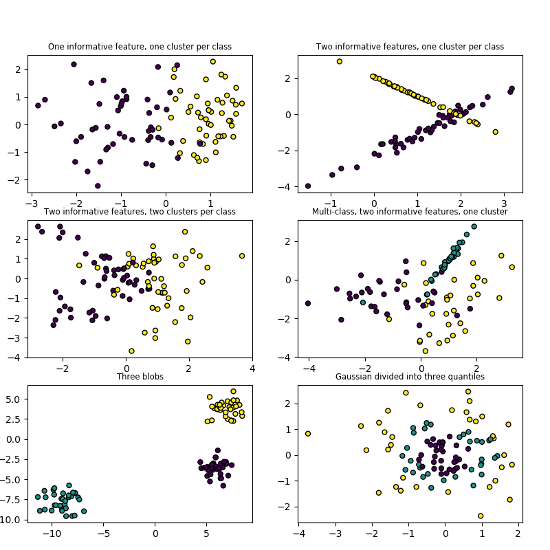
Both make_blobs and make_classification create multiclass datasets by allocating each class one or more normally-distributed clusters of points. make_blobs provides greater control regarding the centers and standard deviations of each cluster, and is used to demonstrate clustering. make_classification specialises in introducing noise by way of: correlated, redundant and uninformative features; multiple Gaussian clusters per class; and linear transformations of the feature space.

make_gaussian_quantiles divides a single Gaussian cluster into near-equal-size classes separated by concentric hyperspheres. make_hastie_10_2 generates a similar binary, 10-dimensional problem.

make_circles and make_moons generate 2d binary classification datasets that are challenging to certain algorithms (e.g. centroid-based clustering or linear classification), including optional Gaussian noise. They are useful for visualisation. produces Gaussian data with a spherical decision boundary for binary classification.

5.4.1.2. Multilabel

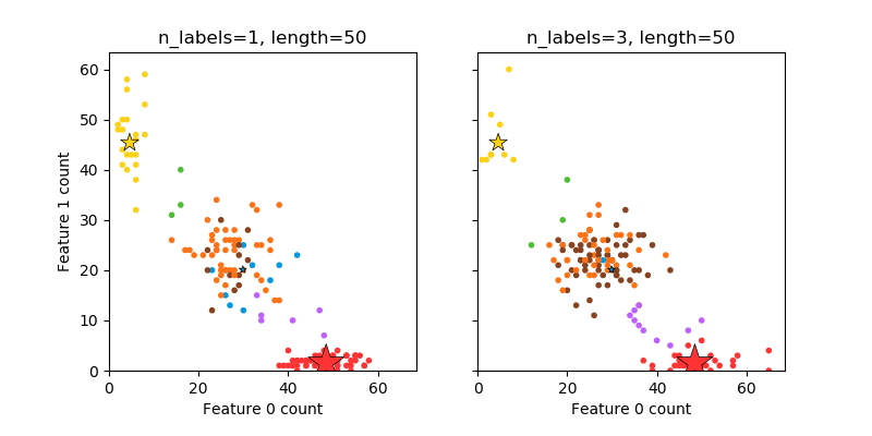
make_multilabel_classification generates random samples with multiple labels, reflecting a bag of words drawn from a mixture of topics. The number of topics for each document is drawn from a Poisson distribution, and the topics themselves are drawn from a fixed random distribution. Similarly, the number of words is drawn from Poisson, with words drawn from a multinomial, where each topic defines a probability distribution over words. Simplifications with respect to true bag-of-words mixtures include:

• Per-topic word distributions are independently drawn, where in reality all would be affected by a sparse base distribution, and would be correlated.
• For a document generated from multiple topics, all topics are weighted equally in generating its bag of words.
• Documents without labels words at random, rather than from a base distribution.

5.4.1.3. Biclustering

make_biclusters(shape, n_clusters[, noise, …])	Generate an array with constant block diagonal structure for biclustering.
make_checkerboard(shape, n_clusters[, …])	Generate an array with block checkerboard structure for biclustering.

5.4.2. Generators for regression

make_regression produces regression targets as an optionally-sparse random linear combination of random features, with noise. Its informative features may be uncorrelated, or low rank (few features account for most of the variance).

Other regression generators generate functions deterministically from randomized features. make_sparse_uncorrelated produces a target as a linear combination of four features with fixed coefficients. Others encode explicitly non-linear relations: make_friedman1 is related by polynomial and sine transforms; make_friedman2 includes feature multiplication and reciprocation; and make_friedman3 is similar with an arctan transformation on the target.

5.4.3. Generators for manifold learning

make_s_curve([n_samples, noise, random_state])	Generate an S curve dataset.
make_swiss_roll([n_samples, noise, random_state])	Generate a swiss roll dataset.

5.4.4. Generators for decomposition

make_low_rank_matrix([n_samples, …])	Generate a mostly low rank matrix with bell-shaped singular values
make_sparse_coded_signal(n_samples, …[, …])	Generate a signal as a sparse combination of dictionary elements.
make_spd_matrix(n_dim[, random_state])	Generate a random symmetric, positive-definite matrix.
make_sparse_spd_matrix([dim, alpha, …])	Generate a sparse symmetric definite positive matrix.

5.5. Loading other datasets

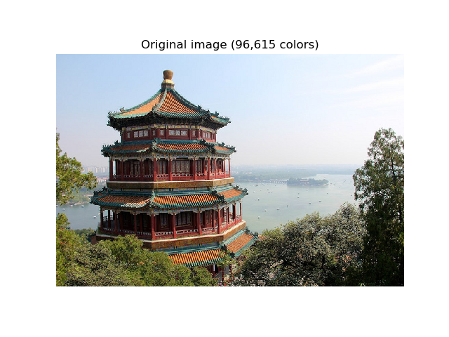
5.5.1. Sample images

Scikit-learn also embed a couple of sample JPEG images published under Creative Commons license by their authors. Those image can be useful to test algorithms and pipeline on 2D data.

load_sample_images()	Load sample images for image manipulation.
load_sample_image(image_name)	Load the numpy array of a single sample image

Warning

The default coding of images is based on the uint8 dtype to spare memory. Often machine learning algorithms work best if the input is converted to a floating point representation first. Also, if you plan to use matplotlib.pyplpt.imshow don’t forget to scale to the range 0 - 1 as done in the following example.

Examples:

• Color Quantization using K-Means

5.5.2. Datasets in svmlight / libsvm format

scikit-learn includes utility functions for loading datasets in the svmlight / libsvm format. In this format, each line takes the form <label> <feature-id>:<feature-value> <feature-id>:<feature-value> .... This format is especially suitable for sparse datasets. In this module, scipy sparse CSR matrices are used for X and numpy arrays are used for y.

You may load a dataset like as follows:

>>> from sklearn.datasets import load_svmlight_file
>>> X_train, y_train = load_svmlight_file("/path/to/train_dataset.txt")
...                                                         

You may also load two (or more) datasets at once:

>>> X_train, y_train, X_test, y_test = load_svmlight_files(
...     ("/path/to/train_dataset.txt", "/path/to/test_dataset.txt"))
...                                                         

In this case, X_train and X_test are guaranteed to have the same number of features. Another way to achieve the same result is to fix the number of features:

>>> X_test, y_test = load_svmlight_file(
...     "/path/to/test_dataset.txt", n_features=X_train.shape[1])
...                                                         

Related links:

Public datasets in svmlight / libsvm format: https://www.csie.ntu.edu.tw/~cjlin/libsvmtools/datasets

Faster API-compatible implementation: https://github.com/mblondel/svmlight-loader

5.5.3. Downloading datasets from the openml.org repository

openml.org is a public repository for machine learning data and experiments, that allows everybody to upload open datasets.

The sklearn.datasets package is able to download datasets from the repository using the function sklearn.datasets.fetch_openml.

For example, to download a dataset of gene expressions in mice brains:

>>> from sklearn.datasets import fetch_openml
>>> mice = fetch_openml(name='miceprotein', version=4)

To fully specify a dataset, you need to provide a name and a version, though the version is optional, see Dataset Versions below. The dataset contains a total of 1080 examples belonging to 8 different classes:

>>> mice.data.shape
(1080, 77)
>>> mice.target.shape
(1080,)
>>> np.unique(mice.target) 
array(['c-CS-m', 'c-CS-s', 'c-SC-m', 'c-SC-s', 't-CS-m', 't-CS-s', 't-SC-m', 't-SC-s'], dtype=object)

You can get more information on the dataset by looking at the DESCR and details attributes:

>>> print(mice.DESCR) 
**Author**: Clara Higuera, Katheleen J. Gardiner, Krzysztof J. Cios
**Source**: [UCI](https://archive.ics.uci.edu/ml/datasets/Mice+Protein+Expression) - 2015
**Please cite**: Higuera C, Gardiner KJ, Cios KJ (2015) Self-Organizing
Feature Maps Identify Proteins Critical to Learning in a Mouse Model of Down
Syndrome. PLoS ONE 10(6): e0129126...

>>> mice.details 
{'id': '40966', 'name': 'MiceProtein', 'version': '4', 'format': 'ARFF',
'upload_date': '2017-11-08T16:00:15', 'licence': 'Public',
'url': 'https://www.openml.org/data/v1/download/17928620/MiceProtein.arff',
'file_id': '17928620', 'default_target_attribute': 'class',
'row_id_attribute': 'MouseID',
'ignore_attribute': ['Genotype', 'Treatment', 'Behavior'],
'tag': ['OpenML-CC18', 'study_135', 'study_98', 'study_99'],
'visibility': 'public', 'status': 'active',
'md5_checksum': '3c479a6885bfa0438971388283a1ce32'}

The DESCR contains a free-text description of the data, while details contains a dictionary of meta-data stored by openml, like the dataset id. For more details, see the OpenML documentation The data_id of the mice protein dataset is 40966, and you can use this (or the name) to get more information on the dataset on the openml website:

>>> mice.url
'https://www.openml.org/d/40966'

The data_id also uniquely identifies a dataset from OpenML:

>>> mice = fetch_openml(data_id=40966)
>>> mice.details 
{'id': '4550', 'name': 'MiceProtein', 'version': '1', 'format': 'ARFF',
'creator': ...,
'upload_date': '2016-02-17T14:32:49', 'licence': 'Public', 'url':
'https://www.openml.org/data/v1/download/1804243/MiceProtein.ARFF', 'file_id':
'1804243', 'default_target_attribute': 'class', 'citation': 'Higuera C,
Gardiner KJ, Cios KJ (2015) Self-Organizing Feature Maps Identify Proteins
Critical to Learning in a Mouse Model of Down Syndrome. PLoS ONE 10(6):
e0129126. [Web Link] journal.pone.0129126', 'tag': ['OpenML100', 'study_14',
'study_34'], 'visibility': 'public', 'status': 'active', 'md5_checksum':
'3c479a6885bfa0438971388283a1ce32'}

5.5.3.1. Dataset Versions

A dataset is uniquely specified by its data_id, but not necessarily by its name. Several different “versions” of a dataset with the same name can exist which can contain entirely different datasets. If a particular version of a dataset has been found to contain significant issues, it might be deactivated. Using a name to specify a dataset will yield the earliest version of a dataset that is still active. That means that fetch_openml(name="miceprotein") can yield different results at different times if earlier versions become inactive. You can see that the dataset with data_id 40966 that we fetched above is the version 1 of the “miceprotein” dataset:

>>> mice.details['version']  
'1'

In fact, this dataset only has one version. The iris dataset on the other hand has multiple versions:

>>> iris = fetch_openml(name="iris")
>>> iris.details['version']  
'1'
>>> iris.details['id']  
'61'

>>> iris_61 = fetch_openml(data_id=61)
>>> iris_61.details['version']
'1'
>>> iris_61.details['id']
'61'

>>> iris_969 = fetch_openml(data_id=969)
>>> iris_969.details['version']
'3'
>>> iris_969.details['id']
'969'

Specifying the dataset by the name “iris” yields the lowest version, version 1, with the data_id 61. To make sure you always get this exact dataset, it is safest to specify it by the dataset data_id. The other dataset, with data_id 969, is version 3 (version 2 has become inactive), and contains a binarized version of the data:

>>> np.unique(iris_969.target)
array(['N', 'P'], dtype=object)

You can also specify both the name and the version, which also uniquely identifies the dataset:

>>> iris_version_3 = fetch_openml(name="iris", version=3)
>>> iris_version_3.details['version']
'3'
>>> iris_version_3.details['id']
'969'

References:

• Vanschoren, van Rijn, Bischl and Torgo “OpenML: networked science in machine learning”, ACM SIGKDD Explorations Newsletter, 15(2), 49-60, 2014.

5.5.4. Loading from external datasets

scikit-learn works on any numeric data stored as numpy arrays or scipy sparse matrices. Other types that are convertible to numeric arrays such as pandas DataFrame are also acceptable.

Here are some recommended ways to load standard columnar data into a format usable by scikit-learn:

• pandas.io provides tools to read data from common formats including CSV, Excel, JSON and SQL. DataFrames may also be constructed from lists of tuples or dicts. Pandas handles heterogeneous data smoothly and provides tools for manipulation and conversion into a numeric array suitable for scikit-learn.
• scipy.io specializes in binary formats often used in scientific computing context such as .mat and .arff
• numpy/routines.io for standard loading of columnar data into numpy arrays
• scikit-learn’s datasets.load_svmlight_file for the svmlight or libSVM sparse format
• scikit-learn’s datasets.load_files for directories of text files where the name of each directory is the name of each category and each file inside of each directory corresponds to one sample from that category

For some miscellaneous data such as images, videos, and audio, you may wish to refer to:

• skimage.io or Imageio for loading images and videos into numpy arrays
• scipy.io.wavfile.read for reading WAV files into a numpy array

Categorical (or nominal) features stored as strings (common in pandas DataFrames) will need converting to numerical features using sklearn.preprocessing.OneHotEncoder or sklearn.preprocessing.OrdinalEncoder or similar. See Preprocessing data.

Note: if you manage your own numerical data it is recommended to use an optimized file format such as HDF5 to reduce data load times. Various libraries such as H5Py, PyTables and pandas provides a Python interface for reading and writing data in that format.