
4.3. Preprocessing data
The sklearn.preprocessing package provides several common
utility functions and transformer classes to change raw feature vectors
into a representation that is more suitable for the downstream estimators.
In general, learning algorithms benefit from standardization of the data set. If some outliers are present in the set, robust scalers or transformers are more appropriate. The behaviors of the different scalers, transformers, and normalizers on a dataset containing marginal outliers is highlighted in Compare the effect of different scalers on data with outliers.
4.3.1. Standardization, or mean removal and variance scaling
Standardization of datasets is a common requirement for many machine learning estimators implemented in scikit-learn; they might behave badly if the individual features do not more or less look like standard normally distributed data: Gaussian with zero mean and unit variance.
In practice we often ignore the shape of the distribution and just transform the data to center it by removing the mean value of each feature, then scale it by dividing non-constant features by their standard deviation.
For instance, many elements used in the objective function of a learning algorithm (such as the RBF kernel of Support Vector Machines or the l1 and l2 regularizers of linear models) assume that all features are centered around zero and have variance in the same order. If a feature has a variance that is orders of magnitude larger than others, it might dominate the objective function and make the estimator unable to learn from other features correctly as expected.
The function scale provides a quick and easy way to perform this
operation on a single array-like dataset:
>>> from sklearn import preprocessing
>>> import numpy as np
>>> X_train = np.array([[ 1., -1.,  2.],
...                     [ 2.,  0.,  0.],
...                     [ 0.,  1., -1.]])
>>> X_scaled = preprocessing.scale(X_train)

>>> X_scaled
array([[ 0.  ..., -1.22...,  1.33...],
       [ 1.22...,  0.  ..., -0.26...],
       [-1.22...,  1.22..., -1.06...]])
Scaled data has zero mean and unit variance:
>>> X_scaled.mean(axis=0)
array([0., 0., 0.])

>>> X_scaled.std(axis=0)
array([1., 1., 1.])
The preprocessing module further provides a utility class
StandardScaler that implements the Transformer API to compute
the mean and standard deviation on a training set so as to be
able to later reapply the same transformation on the testing set.
This class is hence suitable for use in the early steps of a
sklearn.pipeline.Pipeline:
>>> scaler = preprocessing.StandardScaler().fit(X_train)
>>> scaler
StandardScaler(copy=True, with_mean=True, with_std=True)

>>> scaler.mean_
array([1. ..., 0. ..., 0.33...])

>>> scaler.scale_
array([0.81..., 0.81..., 1.24...])

>>> scaler.transform(X_train)
array([[ 0.  ..., -1.22...,  1.33...],
       [ 1.22...,  0.  ..., -0.26...],
       [-1.22...,  1.22..., -1.06...]])
The scaler instance can then be used on new data to transform it the same way it did on the training set:
>>> X_test = [[-1., 1., 0.]]
>>> scaler.transform(X_test)
array([[-2.44...,  1.22..., -0.26...]])
It is possible to disable either centering or scaling by either
passing with_mean=False or with_std=False to the constructor
of StandardScaler.
4.3.1.1. Scaling features to a range
An alternative standardization is scaling features to
lie between a given minimum and maximum value, often between zero and one,
or so that the maximum absolute value of each feature is scaled to unit size.
This can be achieved using MinMaxScaler or MaxAbsScaler,
respectively.
The motivation to use this scaling include robustness to very small standard deviations of features and preserving zero entries in sparse data.
Here is an example to scale a toy data matrix to the [0, 1] range:
>>> X_train = np.array([[ 1., -1.,  2.],
...                     [ 2.,  0.,  0.],
...                     [ 0.,  1., -1.]])
...
>>> min_max_scaler = preprocessing.MinMaxScaler()
>>> X_train_minmax = min_max_scaler.fit_transform(X_train)
>>> X_train_minmax
array([[0.5       , 0.        , 1.        ],
       [1.        , 0.5       , 0.33333333],
       [0.        , 1.        , 0.        ]])
The same instance of the transformer can then be applied to some new test data unseen during the fit call: the same scaling and shifting operations will be applied to be consistent with the transformation performed on the train data:
>>> X_test = np.array([[-3., -1.,  4.]])
>>> X_test_minmax = min_max_scaler.transform(X_test)
>>> X_test_minmax
array([[-1.5       ,  0.        ,  1.66666667]])
It is possible to introspect the scaler attributes to find about the exact nature of the transformation learned on the training data:
>>> min_max_scaler.scale_
array([0.5       , 0.5       , 0.33...])

>>> min_max_scaler.min_
array([0.        , 0.5       , 0.33...])
If MinMaxScaler is given an explicit feature_range=(min, max) the
full formula is:
X_std = (X - X.min(axis=0)) / (X.max(axis=0) - X.min(axis=0))

X_scaled = X_std * (max - min) + min
MaxAbsScaler works in a very similar fashion, but scales in a way
that the training data lies within the range [-1, 1] by dividing through
the largest maximum value in each feature. It is meant for data
that is already centered at zero or sparse data.
Here is how to use the toy data from the previous example with this scaler:
>>> X_train = np.array([[ 1., -1.,  2.],
...                     [ 2.,  0.,  0.],
...                     [ 0.,  1., -1.]])
...
>>> max_abs_scaler = preprocessing.MaxAbsScaler()
>>> X_train_maxabs = max_abs_scaler.fit_transform(X_train)
>>> X_train_maxabs                # doctest +NORMALIZE_WHITESPACE^
array([[ 0.5, -1. ,  1. ],
       [ 1. ,  0. ,  0. ],
       [ 0. ,  1. , -0.5]])
>>> X_test = np.array([[ -3., -1.,  4.]])
>>> X_test_maxabs = max_abs_scaler.transform(X_test)
>>> X_test_maxabs
array([[-1.5, -1. ,  2. ]])
>>> max_abs_scaler.scale_
array([2.,  1.,  2.])
As with scale, the module further provides convenience functions
minmax_scale and maxabs_scale if you don’t want to create
an object.
4.3.1.2. Scaling sparse data
Centering sparse data would destroy the sparseness structure in the data, and thus rarely is a sensible thing to do. However, it can make sense to scale sparse inputs, especially if features are on different scales.
MaxAbsScaler and maxabs_scale were specifically designed
for scaling sparse data, and are the recommended way to go about this.
However, scale and StandardScaler can accept scipy.sparse
matrices as input, as long as with_mean=False is explicitly passed
to the constructor. Otherwise a ValueError will be raised as
silently centering would break the sparsity and would often crash the
execution by allocating excessive amounts of memory unintentionally.
RobustScaler cannot be fitted to sparse inputs, but you can use
the transform method on sparse inputs.
Note that the scalers accept both Compressed Sparse Rows and Compressed
Sparse Columns format (see scipy.sparse.csr_matrix and
scipy.sparse.csc_matrix). Any other sparse input will be converted to
the Compressed Sparse Rows representation. To avoid unnecessary memory
copies, it is recommended to choose the CSR or CSC representation upstream.
Finally, if the centered data is expected to be small enough, explicitly
converting the input to an array using the toarray method of sparse matrices
is another option.
4.3.1.3. Scaling data with outliers
If your data contains many outliers, scaling using the mean and variance
of the data is likely to not work very well. In these cases, you can use
robust_scale and RobustScaler as drop-in replacements
instead. They use more robust estimates for the center and range of your
data.
References:
Further discussion on the importance of centering and scaling data is available on this FAQ: Should I normalize/standardize/rescale the data?
Scaling vs Whitening
It is sometimes not enough to center and scale the features independently, since a downstream model can further make some assumption on the linear independence of the features.
To address this issue you can use sklearn.decomposition.PCA with
whiten=True to further remove the linear correlation across features.
Scaling a 1D array
All above functions (i.e. scale, minmax_scale,
maxabs_scale, and robust_scale) accept 1D array which can be
useful in some specific case.
4.3.1.4. Centering kernel matrices
If you have a kernel matrix of a kernel \(K\) that computes a dot product
in a feature space defined by function \(phi\),
a KernelCenterer can transform the kernel matrix
so that it contains inner products in the feature space
defined by \(phi\) followed by removal of the mean in that space.
4.3.2. Non-linear transformation
4.3.2.1. Mapping to a Uniform distribution
Like scalers, QuantileTransformer puts all features into the same,
known range or distribution. However, by performing a rank transformation, it
smooths out unusual distributions and is less influenced by outliers than
scaling methods. It does, however, distort correlations and distances within
and across features.
QuantileTransformer and quantile_transform provide a
non-parametric transformation based on the quantile function to map the data to
a uniform distribution with values between 0 and 1:
>>> from sklearn.datasets import load_iris
>>> from sklearn.model_selection import train_test_split
>>> iris = load_iris()
>>> X, y = iris.data, iris.target
>>> X_train, X_test, y_train, y_test = train_test_split(X, y, random_state=0)
>>> quantile_transformer = preprocessing.QuantileTransformer(random_state=0)
>>> X_train_trans = quantile_transformer.fit_transform(X_train)
>>> X_test_trans = quantile_transformer.transform(X_test)
>>> np.percentile(X_train[:, 0], [0, 25, 50, 75, 100])
array([ 4.3,  5.1,  5.8,  6.5,  7.9])
This feature corresponds to the sepal length in cm. Once the quantile transformation applied, those landmarks approach closely the percentiles previously defined:
>>> np.percentile(X_train_trans[:, 0], [0, 25, 50, 75, 100])
...
array([ 0.00... ,  0.24...,  0.49...,  0.73...,  0.99... ])
This can be confirmed on a independent testing set with similar remarks:
>>> np.percentile(X_test[:, 0], [0, 25, 50, 75, 100])
...
array([ 4.4  ,  5.125,  5.75 ,  6.175,  7.3  ])
>>> np.percentile(X_test_trans[:, 0], [0, 25, 50, 75, 100])
...
array([ 0.01...,  0.25...,  0.46...,  0.60... ,  0.94...])
4.3.2.2. Mapping to a Gaussian distribution
In many modeling scenarios, normality of the features in a dataset is desirable. Power transforms are a family of parametric, monotonic transformations that aim to map data from any distribution to as close to a Gaussian distribution as possible in order to stabilize variance and minimize skewness.
PowerTransformer currently provides two such power transformations,
the Yeo-Johnson transform and the Box-Cox transform.
The Yeo-Johnson transform is given by:
while the Box-Cox transform is given by:
Box-Cox can only be applied to strictly positive data. In both methods, the transformation is parameterized by \(\lambda\), which is determined through maximum likelihood estimation. Here is an example of using Box-Cox to map samples drawn from a lognormal distribution to a normal distribution:
>>> pt = preprocessing.PowerTransformer(method='box-cox', standardize=False)
>>> X_lognormal = np.random.RandomState(616).lognormal(size=(3, 3))
>>> X_lognormal
array([[1.28..., 1.18..., 0.84...],
       [0.94..., 1.60..., 0.38...],
       [1.35..., 0.21..., 1.09...]])
>>> pt.fit_transform(X_lognormal)
array([[ 0.49...,  0.17..., -0.15...],
       [-0.05...,  0.58..., -0.57...],
       [ 0.69..., -0.84...,  0.10...]])
While the above example sets the standardize option to False,
PowerTransformer will apply zero-mean, unit-variance normalization
to the transformed output by default.
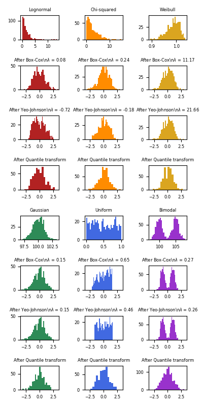
Below are examples of Box-Cox and Yeo-Johnson applied to various probability distributions. Note that when applied to certain distributions, the power transforms achieve very Gaussian-like results, but with others, they are ineffective. This highlights the importance of visualizing the data before and after transformation.
It is also possible to map data to a normal distribution using
QuantileTransformer by setting output_distribution='normal'.
Using the earlier example with the iris dataset:
>>> quantile_transformer = preprocessing.QuantileTransformer(
...     output_distribution='normal', random_state=0)
>>> X_trans = quantile_transformer.fit_transform(X)
>>> quantile_transformer.quantiles_
array([[4.3...,   2...,     1...,     0.1...],
       [4.31...,  2.02...,  1.01...,  0.1...],
       [4.32...,  2.05...,  1.02...,  0.1...],
       ...,
       [7.84...,  4.34...,  6.84...,  2.5...],
       [7.87...,  4.37...,  6.87...,  2.5...],
       [7.9...,   4.4...,   6.9...,   2.5...]])
Thus the median of the input becomes the mean of the output, centered at 0. The normal output is clipped so that the input’s minimum and maximum — corresponding to the 1e-7 and 1 - 1e-7 quantiles respectively — do not become infinite under the transformation.
4.3.3. Normalization
Normalization is the process of scaling individual samples to have unit norm. This process can be useful if you plan to use a quadratic form such as the dot-product or any other kernel to quantify the similarity of any pair of samples.
This assumption is the base of the Vector Space Model often used in text classification and clustering contexts.
The function normalize provides a quick and easy way to perform this
operation on a single array-like dataset, either using the l1 or l2
norms:
>>> X = [[ 1., -1.,  2.],
...      [ 2.,  0.,  0.],
...      [ 0.,  1., -1.]]
>>> X_normalized = preprocessing.normalize(X, norm='l2')

>>> X_normalized
array([[ 0.40..., -0.40...,  0.81...],
       [ 1.  ...,  0.  ...,  0.  ...],
       [ 0.  ...,  0.70..., -0.70...]])
The preprocessing module further provides a utility class
Normalizer that implements the same operation using the
Transformer API (even though the fit method is useless in this case:
the class is stateless as this operation treats samples independently).
This class is hence suitable for use in the early steps of a
sklearn.pipeline.Pipeline:
>>> normalizer = preprocessing.Normalizer().fit(X)  # fit does nothing
>>> normalizer
Normalizer(copy=True, norm='l2')
The normalizer instance can then be used on sample vectors as any transformer:
>>> normalizer.transform(X)
array([[ 0.40..., -0.40...,  0.81...],
       [ 1.  ...,  0.  ...,  0.  ...],
       [ 0.  ...,  0.70..., -0.70...]])

>>> normalizer.transform([[-1.,  1., 0.]])
array([[-0.70...,  0.70...,  0.  ...]])
Sparse input
normalize and Normalizer accept both dense array-like
and sparse matrices from scipy.sparse as input.
For sparse input the data is converted to the Compressed Sparse Rows
representation (see scipy.sparse.csr_matrix) before being fed to
efficient Cython routines. To avoid unnecessary memory copies, it is
recommended to choose the CSR representation upstream.
4.3.4. Encoding categorical features
Often features are not given as continuous values but categorical.
For example a person could have features ["male", "female"],
["from Europe", "from US", "from Asia"],
["uses Firefox", "uses Chrome", "uses Safari", "uses Internet Explorer"].
Such features can be efficiently coded as integers, for instance
["male", "from US", "uses Internet Explorer"] could be expressed as
[0, 1, 3] while ["female", "from Asia", "uses Chrome"] would be
[1, 2, 1].
To convert categorical features to such integer codes, we can use the
OrdinalEncoder. This estimator transforms each categorical feature to one
new feature of integers (0 to n_categories - 1):
>>> enc = preprocessing.OrdinalEncoder()
>>> X = [['male', 'from US', 'uses Safari'], ['female', 'from Europe', 'uses Firefox']]
>>> enc.fit(X)
OrdinalEncoder(categories='auto', dtype=<... 'numpy.float64'>)
>>> enc.transform([['female', 'from US', 'uses Safari']])
array([[0., 1., 1.]])
Such integer representation can, however, not be used directly with all scikit-learn estimators, as these expect continuous input, and would interpret the categories as being ordered, which is often not desired (i.e. the set of browsers was ordered arbitrarily).
Another possibility to convert categorical features to features that can be used
with scikit-learn estimators is to use a one-of-K, also known as one-hot or
dummy encoding.
This type of encoding can be obtained with the OneHotEncoder,
which transforms each categorical feature with
n_categories possible values into n_categories binary features, with
one of them 1, and all others 0.
Continuing the example above:
>>> enc = preprocessing.OneHotEncoder()
>>> X = [['male', 'from US', 'uses Safari'], ['female', 'from Europe', 'uses Firefox']]
>>> enc.fit(X)
OneHotEncoder(categorical_features=None, categories=None,
       dtype=<... 'numpy.float64'>, handle_unknown='error',
       n_values=None, sparse=True)
>>> enc.transform([['female', 'from US', 'uses Safari'],
...                ['male', 'from Europe', 'uses Safari']]).toarray()
array([[1., 0., 0., 1., 0., 1.],
       [0., 1., 1., 0., 0., 1.]])
By default, the values each feature can take is inferred automatically
from the dataset and can be found in the categories_ attribute:
>>> enc.categories_
[array(['female', 'male'], dtype=object), array(['from Europe', 'from US'], dtype=object), array(['uses Firefox', 'uses Safari'], dtype=object)]
It is possible to specify this explicitly using the parameter categories.
There are two genders, four possible continents and four web browsers in our
dataset:
>>> genders = ['female', 'male']
>>> locations = ['from Africa', 'from Asia', 'from Europe', 'from US']
>>> browsers = ['uses Chrome', 'uses Firefox', 'uses IE', 'uses Safari']
>>> enc = preprocessing.OneHotEncoder(categories=[genders, locations, browsers])
>>> # Note that for there are missing categorical values for the 2nd and 3rd
>>> # feature
>>> X = [['male', 'from US', 'uses Safari'], ['female', 'from Europe', 'uses Firefox']]
>>> enc.fit(X)
OneHotEncoder(categorical_features=None,
       categories=[...],
       dtype=<... 'numpy.float64'>, handle_unknown='error',
       n_values=None, sparse=True)
>>> enc.transform([['female', 'from Asia', 'uses Chrome']]).toarray()
array([[1., 0., 0., 1., 0., 0., 1., 0., 0., 0.]])
If there is a possibility that the training data might have missing categorical
features, it can often be better to specify handle_unknown='ignore' instead
of setting the categories manually as above. When
handle_unknown='ignore' is specified and unknown categories are encountered
during transform, no error will be raised but the resulting one-hot encoded
columns for this feature will be all zeros
(handle_unknown='ignore' is only supported for one-hot encoding):
>>> enc = preprocessing.OneHotEncoder(handle_unknown='ignore')
>>> X = [['male', 'from US', 'uses Safari'], ['female', 'from Europe', 'uses Firefox']]
>>> enc.fit(X)
OneHotEncoder(categorical_features=None, categories=None,
       dtype=<... 'numpy.float64'>, handle_unknown='ignore',
       n_values=None, sparse=True)
>>> enc.transform([['female', 'from Asia', 'uses Chrome']]).toarray()
array([[1., 0., 0., 0., 0., 0.]])
See Loading features from dicts for categorical features that are represented as a dict, not as scalars.
4.3.5. Discretization
Discretization (otherwise known as quantization or binning) provides a way to partition continuous features into discrete values. Certain datasets with continuous features may benefit from discretization, because discretization can transform the dataset of continuous attributes to one with only nominal attributes.
One-hot encoded discretized features can make a model more expressive, while maintaining interpretability. For instance, pre-processing with a discretizer can introduce nonlinearity to linear models.
4.3.5.1. K-bins discretization
KBinsDiscretizer discretizers features into k equal width bins:
>>> X = np.array([[ -3., 5., 15 ],
...               [  0., 6., 14 ],
...               [  6., 3., 11 ]])
>>> est = preprocessing.KBinsDiscretizer(n_bins=[3, 2, 2], encode='ordinal').fit(X)
By default the output is one-hot encoded into a sparse matrix
(See Encoding categorical features)
and this can be configured with the encode parameter.
For each feature, the bin edges are computed during fit and together with
the number of bins, they will define the intervals. Therefore, for the current
example, these intervals are defined as:
- feature 1: \({[-\infty, -1), [-1, 2), [2, \infty)}\)
- feature 2: \({[-\infty, 5), [5, \infty)}\)
- feature 3: \({[-\infty, 14), [14, \infty)}\)
Based on these bin intervals,
Xis transformed as follows:>>> est.transform(X) array([[ 0., 1., 1.], [ 1., 1., 1.], [ 2., 0., 0.]])
The resulting dataset contains ordinal attributes which can be further used
in a sklearn.pipeline.Pipeline.
Discretization is similar to constructing histograms for continuous data. However, histograms focus on counting features which fall into particular bins, whereas discretization focuses on assigning feature values to these bins.
KBinsDiscretizer implements different binning strategies, which can be
selected with the strategy parameter. The ‘uniform’ strategy uses
constant-width bins. The ‘quantile’ strategy uses the quantiles values to have
equally populated bins in each feature. The ‘kmeans’ strategy defines bins based
on a k-means clustering procedure performed on each feature independently.
4.3.5.2. Feature binarization
Feature binarization is the process of thresholding numerical
features to get boolean values. This can be useful for downstream
probabilistic estimators that make assumption that the input data
is distributed according to a multi-variate Bernoulli distribution. For instance,
this is the case for the sklearn.neural_network.BernoulliRBM.
It is also common among the text processing community to use binary feature values (probably to simplify the probabilistic reasoning) even if normalized counts (a.k.a. term frequencies) or TF-IDF valued features often perform slightly better in practice.
As for the Normalizer, the utility class
Binarizer is meant to be used in the early stages of
sklearn.pipeline.Pipeline. The fit method does nothing
as each sample is treated independently of others:
>>> X = [[ 1., -1.,  2.],
...      [ 2.,  0.,  0.],
...      [ 0.,  1., -1.]]

>>> binarizer = preprocessing.Binarizer().fit(X)  # fit does nothing
>>> binarizer
Binarizer(copy=True, threshold=0.0)

>>> binarizer.transform(X)
array([[1., 0., 1.],
       [1., 0., 0.],
       [0., 1., 0.]])
It is possible to adjust the threshold of the binarizer:
>>> binarizer = preprocessing.Binarizer(threshold=1.1)
>>> binarizer.transform(X)
array([[0., 0., 1.],
       [1., 0., 0.],
       [0., 0., 0.]])
As for the StandardScaler and Normalizer classes, the
preprocessing module provides a companion function binarize
to be used when the transformer API is not necessary.
Note that the Binarizer is similar to the KBinsDiscretizer
when k = 2, and when the bin edge is at the value threshold.
Sparse input
binarize and Binarizer accept both dense array-like
and sparse matrices from scipy.sparse as input.
For sparse input the data is converted to the Compressed Sparse Rows
representation (see scipy.sparse.csr_matrix).
To avoid unnecessary memory copies, it is recommended to choose the CSR
representation upstream.
4.3.6. Imputation of missing values
Tools for imputing missing values are discussed at Imputation of missing values.
4.3.7. Generating polynomial features
Often it’s useful to add complexity to the model by considering nonlinear features of the input data. A simple and common method to use is polynomial features, which can get features’ high-order and interaction terms. It is implemented in PolynomialFeatures:
>>> import numpy as np
>>> from sklearn.preprocessing import PolynomialFeatures
>>> X = np.arange(6).reshape(3, 2)
>>> X
array([[0, 1],
       [2, 3],
       [4, 5]])
>>> poly = PolynomialFeatures(2)
>>> poly.fit_transform(X)
array([[ 1.,  0.,  1.,  0.,  0.,  1.],
       [ 1.,  2.,  3.,  4.,  6.,  9.],
       [ 1.,  4.,  5., 16., 20., 25.]])
The features of X have been transformed from \((X_1, X_2)\) to \((1, X_1, X_2, X_1^2, X_1X_2, X_2^2)\).
In some cases, only interaction terms among features are required, and it can be gotten with the setting interaction_only=True:
>>> X = np.arange(9).reshape(3, 3)
>>> X
array([[0, 1, 2],
       [3, 4, 5],
       [6, 7, 8]])
>>> poly = PolynomialFeatures(degree=3, interaction_only=True)
>>> poly.fit_transform(X)
array([[  1.,   0.,   1.,   2.,   0.,   0.,   2.,   0.],
       [  1.,   3.,   4.,   5.,  12.,  15.,  20.,  60.],
       [  1.,   6.,   7.,   8.,  42.,  48.,  56., 336.]])
The features of X have been transformed from \((X_1, X_2, X_3)\) to \((1, X_1, X_2, X_3, X_1X_2, X_1X_3, X_2X_3, X_1X_2X_3)\).
Note that polynomial features are used implicitly in kernel methods (e.g., sklearn.svm.SVC, sklearn.decomposition.KernelPCA) when using polynomial Kernel functions.
See Polynomial interpolation for Ridge regression using created polynomial features.
4.3.8. Custom transformers
Often, you will want to convert an existing Python function into a transformer
to assist in data cleaning or processing. You can implement a transformer from
an arbitrary function with FunctionTransformer. For example, to build
a transformer that applies a log transformation in a pipeline, do:
>>> import numpy as np
>>> from sklearn.preprocessing import FunctionTransformer
>>> transformer = FunctionTransformer(np.log1p, validate=True)
>>> X = np.array([[0, 1], [2, 3]])
>>> transformer.transform(X)
array([[0.        , 0.69314718],
       [1.09861229, 1.38629436]])
You can ensure that func and inverse_func are the inverse of each other
by setting check_inverse=True and calling fit before
transform. Please note that a warning is raised and can be turned into an
error with a filterwarnings:
>>> import warnings
>>> warnings.filterwarnings("error", message=".*check_inverse*.",
...                         category=UserWarning, append=False)
For a full code example that demonstrates using a FunctionTransformer
to do custom feature selection,
see Using FunctionTransformer to select columns