
2.7. Novelty and Outlier Detection
Many applications require being able to decide whether a new observation belongs to the same distribution as existing observations (it is an inlier), or should be considered as different (it is an outlier). Often, this ability is used to clean real data sets. Two important distinction must be made:
| novelty detection: | |
|---|---|
| The training data is not polluted by outliers, and we are interested in detecting anomalies in new observations. | |
| outlier detection: | |
| The training data contains outliers, and we need to fit the central mode of the training data, ignoring the deviant observations. | |
The scikit-learn project provides a set of machine learning tools that can be used both for novelty or outliers detection. This strategy is implemented with objects learning in an unsupervised way from the data:
estimator.fit(X_train)
new observations can then be sorted as inliers or outliers with a predict method:
estimator.predict(X_test)
Inliers are labeled 1, while outliers are labeled -1.
2.7.1. Novelty Detection
Consider a data set of  observations from the same
distribution described by
observations from the same
distribution described by  features. Consider now that we
add one more observation to that data set. Is the new observation so
different from the others that we can doubt it is regular? (i.e. does
it come from the same distribution?) Or on the contrary, is it so
similar to the other that we cannot distinguish it from the original
observations? This is the question addressed by the novelty detection
tools and methods.
features. Consider now that we
add one more observation to that data set. Is the new observation so
different from the others that we can doubt it is regular? (i.e. does
it come from the same distribution?) Or on the contrary, is it so
similar to the other that we cannot distinguish it from the original
observations? This is the question addressed by the novelty detection
tools and methods.
In general, it is about to learn a rough, close frontier delimiting
the contour of the initial observations distribution, plotted in
embedding -dimensional space. Then, if further observations
lay within the frontier-delimited subspace, they are considered as
coming from the same population than the initial
observations. Otherwise, if they lay outside the frontier, we can say
that they are abnormal with a given confidence in our assessment.
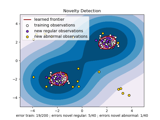
The One-Class SVM has been introduced by Schölkopf et al. for that purpose
and implemented in the Support Vector Machines module in the
svm.OneClassSVM object. It requires the choice of a
kernel and a scalar parameter to define a frontier. The RBF kernel is
usually chosen although there exists no exact formula or algorithm to
set its bandwidth parameter. This is the default in the scikit-learn
implementation. The  parameter, also known as the margin of
the One-Class SVM, corresponds to the probability of finding a new,
but regular, observation outside the frontier.
parameter, also known as the margin of
the One-Class SVM, corresponds to the probability of finding a new,
but regular, observation outside the frontier.
References:
- Estimating the support of a high-dimensional distribution Schölkopf, Bernhard, et al. Neural computation 13.7 (2001): 1443-1471.
Examples:
- See One-class SVM with non-linear kernel (RBF) for visualizing the
frontier learned around some data by a
svm.OneClassSVMobject.
2.7.2. Outlier Detection
Outlier detection is similar to novelty detection in the sense that the goal is to separate a core of regular observations from some polluting ones, called “outliers”. Yet, in the case of outlier detection, we don’t have a clean data set representing the population of regular observations that can be used to train any tool.
2.7.2.1. Fitting an elliptic envelope
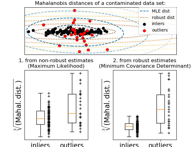
One common way of performing outlier detection is to assume that the regular data come from a known distribution (e.g. data are Gaussian distributed). From this assumption, we generally try to define the “shape” of the data, and can define outlying observations as observations which stand far enough from the fit shape.
The scikit-learn provides an object
covariance.EllipticEnvelope that fits a robust covariance
estimate to the data, and thus fits an ellipse to the central data
points, ignoring points outside the central mode.
For instance, assuming that the inlier data are Gaussian distributed, it will estimate the inlier location and covariance in a robust way (i.e. without being influenced by outliers). The Mahalanobis distances obtained from this estimate is used to derive a measure of outlyingness. This strategy is illustrated below.
Examples:
- See Robust covariance estimation and Mahalanobis distances relevance for
an illustration of the difference between using a standard
(
covariance.EmpiricalCovariance) or a robust estimate (covariance.MinCovDet) of location and covariance to assess the degree of outlyingness of an observation.
References:
- Rousseeuw, P.J., Van Driessen, K. “A fast algorithm for the minimum covariance determinant estimator” Technometrics 41(3), 212 (1999)
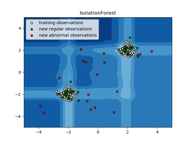
2.7.2.2. Isolation Forest
One efficient way of performing outlier detection in high-dimensional datasets
is to use random forests.
The ensemble.IsolationForest ‘isolates’ observations by randomly selecting
a feature and then randomly selecting a split value between the maximum and
minimum values of the selected feature.
Since recursive partitioning can be represented by a tree structure, the number of splittings required to isolate a sample is equivalent to the path length from the root node to the terminating node.
This path length, averaged over a forest of such random trees, is a measure of normality and our decision function.
Random partitioning produces noticeably shorter paths for anomalies. Hence, when a forest of random trees collectively produce shorter path lengths for particular samples, they are highly likely to be anomalies.
This strategy is illustrated below.
Examples:
- See IsolationForest example for an illustration of the use of IsolationForest.
- See Outlier detection with several methods. for a
comparison of
ensemble.IsolationForestwithneighbors.LocalOutlierFactor,svm.OneClassSVM(tuned to perform like an outlier detection method) and a covariance-based outlier detection withcovariance.EllipticEnvelope.
References:
- Liu, Fei Tony, Ting, Kai Ming and Zhou, Zhi-Hua. “Isolation forest.” Data Mining, 2008. ICDM‘08. Eighth IEEE International Conference on.
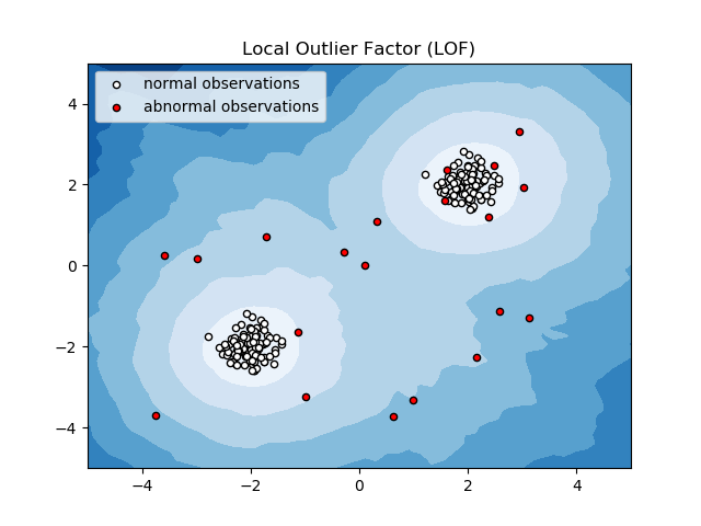
2.7.2.3. Local Outlier Factor
Another efficient way to perform outlier detection on moderately high dimensional datasets is to use the Local Outlier Factor (LOF) algorithm.
The neighbors.LocalOutlierFactor (LOF) algorithm computes a score
(called local outlier factor) reflecting the degree of abnormality of the
observations.
It measures the local density deviation of a given data point with respect to
its neighbors. The idea is to detect the samples that have a substantially
lower density than their neighbors.
In practice the local density is obtained from the k-nearest neighbors. The LOF score of an observation is equal to the ratio of the average local density of his k-nearest neighbors, and its own local density: a normal instance is expected to have a local density similar to that of its neighbors, while abnormal data are expected to have much smaller local density.
The number k of neighbors considered, (alias parameter n_neighbors) is typically chosen 1) greater than the minimum number of objects a cluster has to contain, so that other objects can be local outliers relative to this cluster, and 2) smaller than the maximum number of close by objects that can potentially be local outliers. In practice, such informations are generally not available, and taking n_neighbors=20 appears to work well in general. When the proportion of outliers is high (i.e. greater than 10 %, as in the example below), n_neighbors should be greater (n_neighbors=35 in the example below).
The strength of the LOF algorithm is that it takes both local and global properties of datasets into consideration: it can perform well even in datasets where abnormal samples have different underlying densities. The question is not, how isolated the sample is, but how isolated it is with respect to the surrounding neighborhood.
This strategy is illustrated below.
Examples:
- See Anomaly detection with Local Outlier Factor (LOF) for
an illustration of the use of
neighbors.LocalOutlierFactor. - See Outlier detection with several methods. for a comparison with other anomaly detection methods.
References:
- Breunig, Kriegel, Ng, and Sander (2000) LOF: identifying density-based local outliers. Proc. ACM SIGMOD
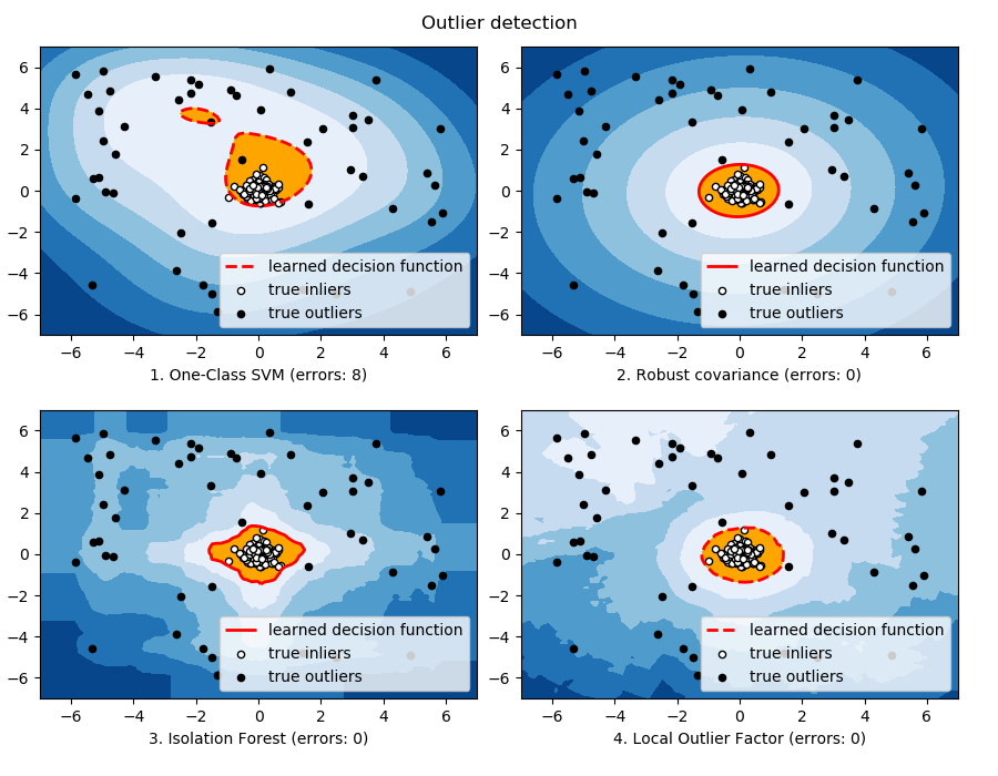
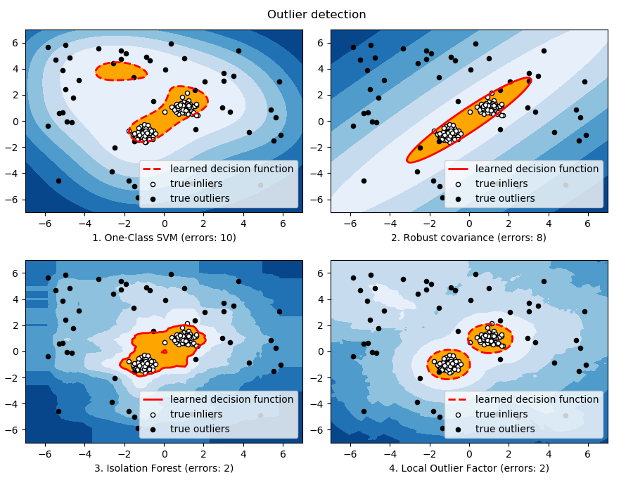
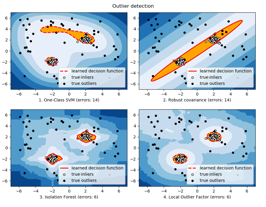
2.7.2.4. One-class SVM versus Elliptic Envelope versus Isolation Forest versus LOF
Strictly-speaking, the One-class SVM is not an outlier-detection method, but a novelty-detection method: its training set should not be contaminated by outliers as it may fit them. That said, outlier detection in high-dimension, or without any assumptions on the distribution of the inlying data is very challenging, and a One-class SVM gives useful results in these situations.
The examples below illustrate how the performance of the
covariance.EllipticEnvelope degrades as the data is less and
less unimodal. The svm.OneClassSVM works better on data with
multiple modes and ensemble.IsolationForest and
neighbors.LocalOutlierFactor perform well in every cases.
For a inlier mode well-centered and elliptic, the
svm.OneClassSVM is not able to benefit from the
rotational symmetry of the inlier population. In addition, it
fits a bit the outliers present in the training set. On the
opposite, the decision rule based on fitting an
covariance.EllipticEnvelope learns an ellipse, which
fits well the inlier distribution. The ensemble.IsolationForest
and neighbors.LocalOutlierFactor perform as well. |
 |
As the inlier distribution becomes bimodal, the
covariance.EllipticEnvelope does not fit well the
inliers. However, we can see that ensemble.IsolationForest,
svm.OneClassSVM and neighbors.LocalOutlierFactor
have difficulties to detect the two modes,
and that the svm.OneClassSVM
tends to overfit: because it has no model of inliers, it
interprets a region where, by chance some outliers are
clustered, as inliers. |
 |
If the inlier distribution is strongly non Gaussian, the
svm.OneClassSVM is able to recover a reasonable
approximation as well as ensemble.IsolationForest
and neighbors.LocalOutlierFactor,
whereas the covariance.EllipticEnvelope completely fails. |
 |
Examples:
- See Outlier detection with several methods. for a
comparison of the
svm.OneClassSVM(tuned to perform like an outlier detection method), theensemble.IsolationForest, theneighbors.LocalOutlierFactorand a covariance-based outlier detectioncovariance.EllipticEnvelope.