sklearn.neighbors.LocalOutlierFactor
-
class
sklearn.neighbors.LocalOutlierFactor(n_neighbors=20, algorithm=’auto’, leaf_size=30, metric=’minkowski’, p=2, metric_params=None, contamination=0.1, n_jobs=1)[source]¶ Unsupervised Outlier Detection using Local Outlier Factor (LOF)
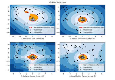
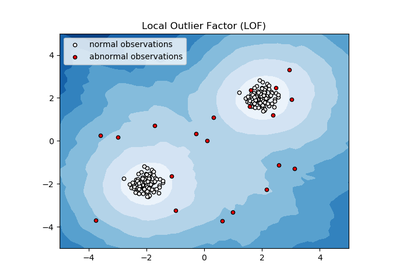
The anomaly score of each sample is called Local Outlier Factor. It measures the local deviation of density of a given sample with respect to its neighbors. It is local in that the anomaly score depends on how isolated the object is with respect to the surrounding neighborhood. More precisely, locality is given by k-nearest neighbors, whose distance is used to estimate the local density. By comparing the local density of a sample to the local densities of its neighbors, one can identify samples that have a substantially lower density than their neighbors. These are considered outliers.
Parameters: n_neighbors : int, optional (default=20)
Number of neighbors to use by default for
kneighborsqueries. If n_neighbors is larger than the number of samples provided, all samples will be used.algorithm : {‘auto’, ‘ball_tree’, ‘kd_tree’, ‘brute’}, optional
Algorithm used to compute the nearest neighbors:
- ‘ball_tree’ will use
BallTree - ‘kd_tree’ will use
KDTree - ‘brute’ will use a brute-force search.
- ‘auto’ will attempt to decide the most appropriate algorithm
based on the values passed to
fitmethod.
Note: fitting on sparse input will override the setting of this parameter, using brute force.
leaf_size : int, optional (default=30)
metric : string or callable, default ‘minkowski’
metric used for the distance computation. Any metric from scikit-learn or scipy.spatial.distance can be used.
If ‘precomputed’, the training input X is expected to be a distance matrix.
If metric is a callable function, it is called on each pair of instances (rows) and the resulting value recorded. The callable should take two arrays as input and return one value indicating the distance between them. This works for Scipy’s metrics, but is less efficient than passing the metric name as a string.
Valid values for metric are:
- from scikit-learn: [‘cityblock’, ‘cosine’, ‘euclidean’, ‘l1’, ‘l2’, ‘manhattan’]
- from scipy.spatial.distance: [‘braycurtis’, ‘canberra’, ‘chebyshev’, ‘correlation’, ‘dice’, ‘hamming’, ‘jaccard’, ‘kulsinski’, ‘mahalanobis’, ‘matching’, ‘minkowski’, ‘rogerstanimoto’, ‘russellrao’, ‘seuclidean’, ‘sokalmichener’, ‘sokalsneath’, ‘sqeuclidean’, ‘yule’]
See the documentation for scipy.spatial.distance for details on these metrics: http://docs.scipy.org/doc/scipy/reference/spatial.distance.html
p : integer, optional (default=2)
Parameter for the Minkowski metric from
sklearn.metrics.pairwise.pairwise_distances. When p = 1, this is equivalent to using manhattan_distance (l1), and euclidean_distance (l2) for p = 2. For arbitrary p, minkowski_distance (l_p) is used.metric_params : dict, optional (default=None)
Additional keyword arguments for the metric function.
contamination : float in (0., 0.5), optional (default=0.1)
The amount of contamination of the data set, i.e. the proportion of outliers in the data set. When fitting this is used to define the threshold on the decision function.
n_jobs : int, optional (default=1)
The number of parallel jobs to run for neighbors search. If
-1, then the number of jobs is set to the number of CPU cores. Affects onlykneighborsandkneighbors_graphmethods.Attributes: negative_outlier_factor_ : numpy array, shape (n_samples,)
The opposite LOF of the training samples. The lower, the more abnormal. Inliers tend to have a LOF score close to 1, while outliers tend to have a larger LOF score.
The local outlier factor (LOF) of a sample captures its supposed ‘degree of abnormality’. It is the average of the ratio of the local reachability density of a sample and those of its k-nearest neighbors.
n_neighbors_ : integer
The actual number of neighbors used for
kneighborsqueries.References
[R243] Breunig, M. M., Kriegel, H. P., Ng, R. T., & Sander, J. (2000, May). LOF: identifying density-based local outliers. In ACM sigmod record. Methods
fit(X[, y])Fit the model using X as training data. fit_predict(X[, y])“Fits the model to the training set X and returns the labels get_params([deep])Get parameters for this estimator. kneighbors([X, n_neighbors, return_distance])Finds the K-neighbors of a point. kneighbors_graph([X, n_neighbors, mode])Computes the (weighted) graph of k-Neighbors for points in X set_params(**params)Set the parameters of this estimator. -
__init__(n_neighbors=20, algorithm=’auto’, leaf_size=30, metric=’minkowski’, p=2, metric_params=None, contamination=0.1, n_jobs=1)[source]
-
fit(X, y=None)[source]¶ Fit the model using X as training data.
Parameters: X : {array-like, sparse matrix, BallTree, KDTree}
Training data. If array or matrix, shape [n_samples, n_features], or [n_samples, n_samples] if metric=’precomputed’.
Returns: self : object
Returns self.
-
fit_predict(X, y=None)[source]¶ “Fits the model to the training set X and returns the labels (1 inlier, -1 outlier) on the training set according to the LOF score and the contamination parameter.
Parameters: X : array-like, shape (n_samples, n_features), default=None
The query sample or samples to compute the Local Outlier Factor w.r.t. to the training samples.
Returns: is_inlier : array, shape (n_samples,)
Returns -1 for anomalies/outliers and 1 for inliers.
-
get_params(deep=True)[source]¶ Get parameters for this estimator.
Parameters: deep : boolean, optional
If True, will return the parameters for this estimator and contained subobjects that are estimators.
Returns: params : mapping of string to any
Parameter names mapped to their values.
-
kneighbors(X=None, n_neighbors=None, return_distance=True)[source]¶ Finds the K-neighbors of a point.
Returns indices of and distances to the neighbors of each point.
Parameters: X : array-like, shape (n_query, n_features), or (n_query, n_indexed) if metric == ‘precomputed’
The query point or points. If not provided, neighbors of each indexed point are returned. In this case, the query point is not considered its own neighbor.
n_neighbors : int
Number of neighbors to get (default is the value passed to the constructor).
return_distance : boolean, optional. Defaults to True.
If False, distances will not be returned
Returns: dist : array
Array representing the lengths to points, only present if return_distance=True
ind : array
Indices of the nearest points in the population matrix.
Examples
In the following example, we construct a NeighborsClassifier class from an array representing our data set and ask who’s the closest point to [1,1,1]
>>> samples = [[0., 0., 0.], [0., .5, 0.], [1., 1., .5]]
>>> from sklearn.neighbors import NearestNeighbors
>>> neigh = NearestNeighbors(n_neighbors=1)
>>> neigh.fit(samples)
NearestNeighbors(algorithm='auto', leaf_size=30, ...)
>>> print(neigh.kneighbors([[1., 1., 1.]]))
(array([[ 0.5]]), array([[2]]...))
As you can see, it returns [[0.5]], and [[2]], which means that the element is at distance 0.5 and is the third element of samples (indexes start at 0). You can also query for multiple points:
>>> X = [[0., 1., 0.], [1., 0., 1.]]
>>> neigh.kneighbors(X, return_distance=False)
array([[1],
       [2]]...)
-
kneighbors_graph(X=None, n_neighbors=None, mode=’connectivity’)[source]¶ Computes the (weighted) graph of k-Neighbors for points in X
Parameters: X : array-like, shape (n_query, n_features), or (n_query, n_indexed) if metric == ‘precomputed’
The query point or points. If not provided, neighbors of each indexed point are returned. In this case, the query point is not considered its own neighbor.
n_neighbors : int
Number of neighbors for each sample. (default is value passed to the constructor).
mode : {‘connectivity’, ‘distance’}, optional
Type of returned matrix: ‘connectivity’ will return the connectivity matrix with ones and zeros, in ‘distance’ the edges are Euclidean distance between points.
Returns: A : sparse matrix in CSR format, shape = [n_samples, n_samples_fit]
n_samples_fit is the number of samples in the fitted data A[i, j] is assigned the weight of edge that connects i to j.
Examples
>>> X = [[0], [3], [1]]
>>> from sklearn.neighbors import NearestNeighbors
>>> neigh = NearestNeighbors(n_neighbors=2)
>>> neigh.fit(X)
NearestNeighbors(algorithm='auto', leaf_size=30, ...)
>>> A = neigh.kneighbors_graph(X)
>>> A.toarray()
array([[ 1.,  0.,  1.],
       [ 0.,  1.,  1.],
       [ 1.,  0.,  1.]])
-
set_params(**params)[source]¶ Set the parameters of this estimator.
The method works on simple estimators as well as on nested objects (such as pipelines). The latter have parameters of the form
<component>__<parameter>so that it’s possible to update each component of a nested object.Returns: self :
- ‘ball_tree’ will use