Note
Go to the end to download the full example code or to run this example in your browser via JupyterLite or Binder
SVM Tie Breaking Example
Tie breaking is costly if decision_function_shape='ovr', and therefore it
is not enabled by default. This example illustrates the effect of the
break_ties parameter for a multiclass classification problem and
decision_function_shape='ovr'.
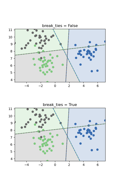
The two plots differ only in the area in the middle where the classes are
tied. If break_ties=False, all input in that area would be classified as
one class, whereas if break_ties=True, the tie-breaking mechanism will
create a non-convex decision boundary in that area.
# Code source: Andreas Mueller, Adrin Jalali
# License: BSD 3 clause

import matplotlib.pyplot as plt
import numpy as np

from sklearn.datasets import make_blobs
from sklearn.svm import SVC

X, y = make_blobs(random_state=27)

fig, sub = plt.subplots(2, 1, figsize=(5, 8))
titles = ("break_ties = False", "break_ties = True")

for break_ties, title, ax in zip((False, True), titles, sub.flatten()):
    svm = SVC(
        kernel="linear", C=1, break_ties=break_ties, decision_function_shape="ovr"
    ).fit(X, y)

    xlim = [X[:, 0].min(), X[:, 0].max()]
    ylim = [X[:, 1].min(), X[:, 1].max()]

    xs = np.linspace(xlim[0], xlim[1], 1000)
    ys = np.linspace(ylim[0], ylim[1], 1000)
    xx, yy = np.meshgrid(xs, ys)

    pred = svm.predict(np.c_[xx.ravel(), yy.ravel()])

    colors = [plt.cm.Accent(i) for i in [0, 4, 7]]

    points = ax.scatter(X[:, 0], X[:, 1], c=y, cmap="Accent")
    classes = [(0, 1), (0, 2), (1, 2)]
    line = np.linspace(X[:, 1].min() - 5, X[:, 1].max() + 5)
    ax.imshow(
        -pred.reshape(xx.shape),
        cmap="Accent",
        alpha=0.2,
        extent=(xlim[0], xlim[1], ylim[1], ylim[0]),
    )

    for coef, intercept, col in zip(svm.coef_, svm.intercept_, classes):
        line2 = -(line * coef[1] + intercept) / coef[0]
        ax.plot(line2, line, "-", c=colors[col[0]])
        ax.plot(line2, line, "--", c=colors[col[1]])
    ax.set_xlim(xlim)
    ax.set_ylim(ylim)
    ax.set_title(title)
    ax.set_aspect("equal")

plt.show()
Total running time of the script: (0 minutes 0.944 seconds)
Related examples
Plot multinomial and One-vs-Rest Logistic Regression
