Note
Go to the end to download the full example code or to run this example in your browser via JupyterLite or Binder
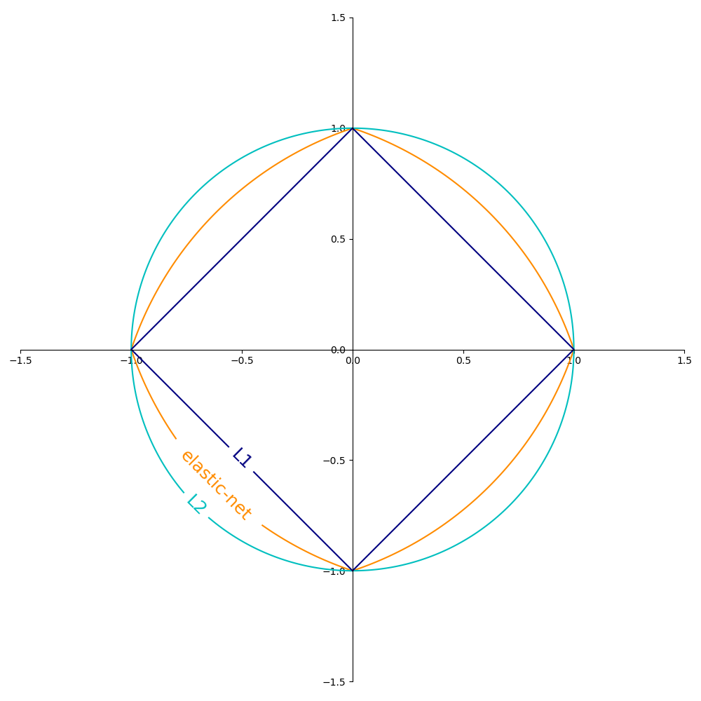
SGD: Penalties
Contours of where the penalty is equal to 1 for the three penalties L1, L2 and elastic-net.
All of the above are supported by SGDClassifier
and SGDRegressor.
import matplotlib.pyplot as plt
import numpy as np

l1_color = "navy"
l2_color = "c"
elastic_net_color = "darkorange"

line = np.linspace(-1.5, 1.5, 1001)
xx, yy = np.meshgrid(line, line)

l2 = xx**2 + yy**2
l1 = np.abs(xx) + np.abs(yy)
rho = 0.5
elastic_net = rho * l1 + (1 - rho) * l2

plt.figure(figsize=(10, 10), dpi=100)
ax = plt.gca()

elastic_net_contour = plt.contour(
    xx, yy, elastic_net, levels=[1], colors=elastic_net_color
)
l2_contour = plt.contour(xx, yy, l2, levels=[1], colors=l2_color)
l1_contour = plt.contour(xx, yy, l1, levels=[1], colors=l1_color)
ax.set_aspect("equal")
ax.spines["left"].set_position("center")
ax.spines["right"].set_color("none")
ax.spines["bottom"].set_position("center")
ax.spines["top"].set_color("none")

plt.clabel(
    elastic_net_contour,
    inline=1,
    fontsize=18,
    fmt={1.0: "elastic-net"},
    manual=[(-1, -1)],
)
plt.clabel(l2_contour, inline=1, fontsize=18, fmt={1.0: "L2"}, manual=[(-1, -1)])
plt.clabel(l1_contour, inline=1, fontsize=18, fmt={1.0: "L1"}, manual=[(-1, -1)])

plt.tight_layout()
plt.show()
Total running time of the script: (0 minutes 0.263 seconds)
Related examples
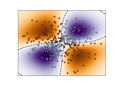
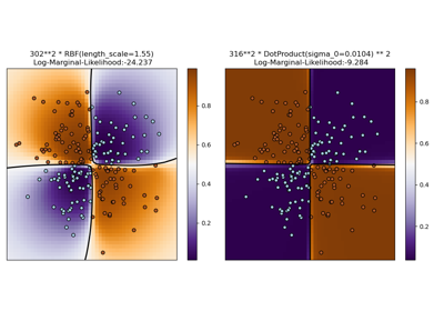
Illustration of Gaussian process classification (GPC) on the XOR dataset
Illustration of Gaussian process classification (GPC) on the XOR dataset