Lasso model selection via information criteria

This example reproduces the example of Fig. 2 of [ZHT2007]. A LassoLarsIC estimator is fit on a diabetes dataset and the AIC and the BIC criteria are used to select the best model.

Note

It is important to note that the optimization to find alpha with LassoLarsIC relies on the AIC or BIC criteria that are computed in-sample, thus on the training set directly. This approach differs from the cross-validation procedure. For a comparison of the two approaches, you can refer to the following example: Lasso model selection: AIC-BIC / cross-validation.

References

[ZHT2007] (1,2)

Zou, Hui, Trevor Hastie, and Robert Tibshirani. “On the degrees of freedom of the lasso.” The Annals of Statistics 35.5 (2007): 2173-2192.

# Author: Alexandre Gramfort
#         Guillaume Lemaitre
# License: BSD 3 clause

We will use the diabetes dataset.

from sklearn.datasets import load_diabetes

X, y = load_diabetes(return_X_y=True, as_frame=True)
n_samples = X.shape[0]
X.head()

	age	sex	bmi	bp	s1	s2	s3	s4	s5	s6
0	0.038076	0.050680	0.061696	0.021872	-0.044223	-0.034821	-0.043401	-0.002592	0.019907	-0.017646
1	-0.001882	-0.044642	-0.051474	-0.026328	-0.008449	-0.019163	0.074412	-0.039493	-0.068332	-0.092204
2	0.085299	0.050680	0.044451	-0.005670	-0.045599	-0.034194	-0.032356	-0.002592	0.002861	-0.025930
3	-0.089063	-0.044642	-0.011595	-0.036656	0.012191	0.024991	-0.036038	0.034309	0.022688	-0.009362
4	0.005383	-0.044642	-0.036385	0.021872	0.003935	0.015596	0.008142	-0.002592	-0.031988	-0.046641

Scikit-learn provides an estimator called LassoLarsIC that uses either Akaike’s information criterion (AIC) or the Bayesian information criterion (BIC) to select the best model. Before fitting this model, we will scale the dataset.

In the following, we are going to fit two models to compare the values reported by AIC and BIC.

from sklearn.linear_model import LassoLarsIC
from sklearn.pipeline import make_pipeline
from sklearn.preprocessing import StandardScaler

lasso_lars_ic = make_pipeline(StandardScaler(), LassoLarsIC(criterion="aic")).fit(X, y)

To be in line with the definition in [ZHT2007], we need to rescale the AIC and the BIC. Indeed, Zou et al. are ignoring some constant terms compared to the original definition of AIC derived from the maximum log-likelihood of a linear model. You can refer to mathematical detail section for the User Guide.

def zou_et_al_criterion_rescaling(criterion, n_samples, noise_variance):
    """Rescale the information criterion to follow the definition of Zou et al."""
    return criterion - n_samples * np.log(2 * np.pi * noise_variance) - n_samples

import numpy as np

aic_criterion = zou_et_al_criterion_rescaling(
    lasso_lars_ic[-1].criterion_,
    n_samples,
    lasso_lars_ic[-1].noise_variance_,
)

index_alpha_path_aic = np.flatnonzero(
    lasso_lars_ic[-1].alphas_ == lasso_lars_ic[-1].alpha_
)[0]

lasso_lars_ic.set_params(lassolarsic__criterion="bic").fit(X, y)

bic_criterion = zou_et_al_criterion_rescaling(
    lasso_lars_ic[-1].criterion_,
    n_samples,
    lasso_lars_ic[-1].noise_variance_,
)

index_alpha_path_bic = np.flatnonzero(
    lasso_lars_ic[-1].alphas_ == lasso_lars_ic[-1].alpha_
)[0]

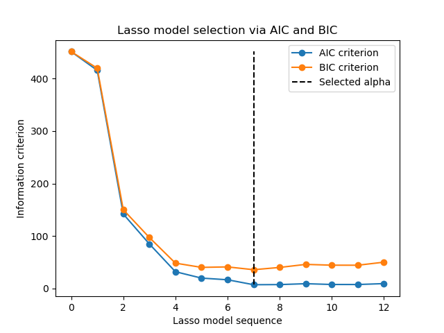
Now that we collected the AIC and BIC, we can as well check that the minima of both criteria happen at the same alpha. Then, we can simplify the following plot.

index_alpha_path_aic == index_alpha_path_bic

True

Finally, we can plot the AIC and BIC criterion and the subsequent selected regularization parameter.

import matplotlib.pyplot as plt

plt.plot(aic_criterion, color="tab:blue", marker="o", label="AIC criterion")
plt.plot(bic_criterion, color="tab:orange", marker="o", label="BIC criterion")
plt.vlines(
    index_alpha_path_bic,
    aic_criterion.min(),
    aic_criterion.max(),
    color="black",
    linestyle="--",
    label="Selected alpha",
)
plt.legend()
plt.ylabel("Information criterion")
plt.xlabel("Lasso model sequence")
_ = plt.title("Lasso model selection via AIC and BIC")