`sklearn.neural_network`.MLPRegressor¶

class sklearn.neural_network.MLPRegressor(hidden_layer_sizes=(100,), activation='relu', *, solver='adam', alpha=0.0001, batch_size='auto', learning_rate='constant', learning_rate_init=0.001, power_t=0.5, max_iter=200, shuffle=True, random_state=None, tol=0.0001, verbose=False, warm_start=False, momentum=0.9, nesterovs_momentum=True, early_stopping=False, validation_fraction=0.1, beta_1=0.9, beta_2=0.999, epsilon=1e-08, n_iter_no_change=10, max_fun=15000)[source]¶

Multi-layer Perceptron regressor.

This model optimizes the squared error using LBFGS or stochastic gradient descent.

New in version 0.18.

Parameters:

hidden_layer_sizesarray-like of shape(n_layers - 2,), default=(100,)

The ith element represents the number of neurons in the ith hidden layer.

activation{‘identity’, ‘logistic’, ‘tanh’, ‘relu’}, default=’relu’

Activation function for the hidden layer.

‘identity’, no-op activation, useful to implement linear bottleneck, returns f(x) = x
‘logistic’, the logistic sigmoid function, returns f(x) = 1 / (1 + exp(-x)).
‘tanh’, the hyperbolic tan function, returns f(x) = tanh(x).
‘relu’, the rectified linear unit function, returns f(x) = max(0, x)

solver{‘lbfgs’, ‘sgd’, ‘adam’}, default=’adam’

The solver for weight optimization.

‘lbfgs’ is an optimizer in the family of quasi-Newton methods.
‘sgd’ refers to stochastic gradient descent.
‘adam’ refers to a stochastic gradient-based optimizer proposed by Kingma, Diederik, and Jimmy Ba

Note: The default solver ‘adam’ works pretty well on relatively large datasets (with thousands of training samples or more) in terms of both training time and validation score. For small datasets, however, ‘lbfgs’ can converge faster and perform better.

alphafloat, default=0.0001

Strength of the L2 regularization term. The L2 regularization term is divided by the sample size when added to the loss.

batch_sizeint, default=’auto’

Size of minibatches for stochastic optimizers. If the solver is ‘lbfgs’, the regressor will not use minibatch. When set to “auto”, batch_size=min(200, n_samples).

learning_rate{‘constant’, ‘invscaling’, ‘adaptive’}, default=’constant’

Learning rate schedule for weight updates.

‘constant’ is a constant learning rate given by ‘learning_rate_init’.
‘invscaling’ gradually decreases the learning rate learning_rate_ at each time step ‘t’ using an inverse scaling exponent of ‘power_t’. effective_learning_rate = learning_rate_init / pow(t, power_t)
‘adaptive’ keeps the learning rate constant to ‘learning_rate_init’ as long as training loss keeps decreasing. Each time two consecutive epochs fail to decrease training loss by at least tol, or fail to increase validation score by at least tol if ‘early_stopping’ is on, the current learning rate is divided by 5.

Only used when solver=’sgd’.

learning_rate_initfloat, default=0.001

The initial learning rate used. It controls the step-size in updating the weights. Only used when solver=’sgd’ or ‘adam’.

power_tfloat, default=0.5

The exponent for inverse scaling learning rate. It is used in updating effective learning rate when the learning_rate is set to ‘invscaling’. Only used when solver=’sgd’.

max_iterint, default=200

Maximum number of iterations. The solver iterates until convergence (determined by ‘tol’) or this number of iterations. For stochastic solvers (‘sgd’, ‘adam’), note that this determines the number of epochs (how many times each data point will be used), not the number of gradient steps.

shufflebool, default=True

Whether to shuffle samples in each iteration. Only used when solver=’sgd’ or ‘adam’.

random_stateint, RandomState instance, default=None

Determines random number generation for weights and bias initialization, train-test split if early stopping is used, and batch sampling when solver=’sgd’ or ‘adam’. Pass an int for reproducible results across multiple function calls. See Glossary.

tolfloat, default=1e-4

Tolerance for the optimization. When the loss or score is not improving by at least tol for n_iter_no_change consecutive iterations, unless learning_rate is set to ‘adaptive’, convergence is considered to be reached and training stops.

verbosebool, default=False

Whether to print progress messages to stdout.

warm_startbool, default=False

When set to True, reuse the solution of the previous call to fit as initialization, otherwise, just erase the previous solution. See the Glossary.

momentumfloat, default=0.9

Momentum for gradient descent update. Should be between 0 and 1. Only used when solver=’sgd’.

nesterovs_momentumbool, default=True

Whether to use Nesterov’s momentum. Only used when solver=’sgd’ and momentum > 0.

early_stoppingbool, default=False

Whether to use early stopping to terminate training when validation score is not improving. If set to True, it will automatically set aside validation_fraction of training data as validation and terminate training when validation score is not improving by at least tol for n_iter_no_change consecutive epochs. Only effective when solver=’sgd’ or ‘adam’.

validation_fractionfloat, default=0.1

The proportion of training data to set aside as validation set for early stopping. Must be between 0 and 1. Only used if early_stopping is True.

beta_1float, default=0.9

Exponential decay rate for estimates of first moment vector in adam, should be in [0, 1). Only used when solver=’adam’.

beta_2float, default=0.999

Exponential decay rate for estimates of second moment vector in adam, should be in [0, 1). Only used when solver=’adam’.

epsilonfloat, default=1e-8

Value for numerical stability in adam. Only used when solver=’adam’.

n_iter_no_changeint, default=10

Maximum number of epochs to not meet tol improvement. Only effective when solver=’sgd’ or ‘adam’.

New in version 0.20.

max_funint, default=15000

Only used when solver=’lbfgs’. Maximum number of function calls. The solver iterates until convergence (determined by tol), number of iterations reaches max_iter, or this number of function calls. Note that number of function calls will be greater than or equal to the number of iterations for the MLPRegressor.

New in version 0.22.

Attributes:

loss_float: The current loss computed with the loss function.
best_loss_float: The minimum loss reached by the solver throughout fitting. If early_stopping=True, this attribute is set to None. Refer to the best_validation_score_ fitted attribute instead. Only accessible when solver=’sgd’ or ‘adam’.
loss_curve_list of shape (n_iter_,): Loss value evaluated at the end of each training step. The ith element in the list represents the loss at the ith iteration. Only accessible when solver=’sgd’ or ‘adam’.
validation_scores_list of shape (n_iter_,) or None: The score at each iteration on a held-out validation set. The score reported is the R2 score. Only available if early_stopping=True, otherwise the attribute is set to None. Only accessible when solver=’sgd’ or ‘adam’.
best_validation_score_float or None: The best validation score (i.e. R2 score) that triggered the early stopping. Only available if early_stopping=True, otherwise the attribute is set to None. Only accessible when solver=’sgd’ or ‘adam’.
t_int: The number of training samples seen by the solver during fitting. Mathematically equals n_iters * X.shape[0], it means time_step and it is used by optimizer’s learning rate scheduler.
coefs_list of shape (n_layers - 1,): The ith element in the list represents the weight matrix corresponding to layer i.
intercepts_list of shape (n_layers - 1,): The ith element in the list represents the bias vector corresponding to layer i + 1.
n_features_in_int: Number of features seen during fit.

New in version 0.24.
feature_names_in_ndarray of shape (n_features_in_,): Names of features seen during fit. Defined only when X has feature names that are all strings.

New in version 1.0.
n_iter_int: The number of iterations the solver has run.
n_layers_int: Number of layers.
n_outputs_int: Number of outputs.
out_activation_str: Name of the output activation function.

See also

BernoulliRBM: Bernoulli Restricted Boltzmann Machine (RBM).
MLPClassifier: Multi-layer Perceptron classifier.
sklearn.linear_model.SGDRegressor: Linear model fitted by minimizing a regularized empirical loss with SGD.

Notes

MLPRegressor trains iteratively since at each time step the partial derivatives of the loss function with respect to the model parameters are computed to update the parameters.

It can also have a regularization term added to the loss function that shrinks model parameters to prevent overfitting.

This implementation works with data represented as dense and sparse numpy arrays of floating point values.

References

Hinton, Geoffrey E. “Connectionist learning procedures.” Artificial intelligence 40.1 (1989): 185-234.

Glorot, Xavier, and Yoshua Bengio. “Understanding the difficulty of training deep feedforward neural networks.” International Conference on Artificial Intelligence and Statistics. 2010.

He, Kaiming, et al (2015). “Delving deep into rectifiers: Surpassing human-level performance on imagenet classification.”

Kingma, Diederik, and Jimmy Ba (2014) “Adam: A method for stochastic optimization.”

Examples

>>> from sklearn.neural_network import MLPRegressor
>>> from sklearn.datasets import make_regression
>>> from sklearn.model_selection import train_test_split
>>> X, y = make_regression(n_samples=200, random_state=1)
>>> X_train, X_test, y_train, y_test = train_test_split(X, y,
...                                                     random_state=1)
>>> regr = MLPRegressor(random_state=1, max_iter=500).fit(X_train, y_train)
>>> regr.predict(X_test[:2])
array([-0.9..., -7.1...])
>>> regr.score(X_test, y_test)
0.4...

Methods

`fit`(X, y)	Fit the model to data matrix X and target(s) y.
`get_params`([deep])	Get parameters for this estimator.
`partial_fit`(X, y)	Update the model with a single iteration over the given data.
`predict`(X)	Predict using the multi-layer perceptron model.
`score`(X, y[, sample_weight])	Return the coefficient of determination of the prediction.
`set_params`(**params)	Set the parameters of this estimator.

fit(X, y)[source]¶

Fit the model to data matrix X and target(s) y.

Parameters:

Xndarray or sparse matrix of shape (n_samples, n_features): The input data.
yndarray of shape (n_samples,) or (n_samples, n_outputs): The target values (class labels in classification, real numbers in regression).

Returns:

selfobject: Returns a trained MLP model.

get_params(deep=True)[source]¶

Get parameters for this estimator.

Parameters:

deepbool, default=True: If True, will return the parameters for this estimator and contained subobjects that are estimators.

Returns:

paramsdict: Parameter names mapped to their values.

partial_fit(X, y)[source]¶

Update the model with a single iteration over the given data.

Parameters:

X{array-like, sparse matrix} of shape (n_samples, n_features): The input data.
yndarray of shape (n_samples,): The target values.

Returns:

selfobject: Trained MLP model.

predict(X)[source]¶

Predict using the multi-layer perceptron model.

Parameters:

X{array-like, sparse matrix} of shape (n_samples, n_features): The input data.

Returns:

yndarray of shape (n_samples, n_outputs): The predicted values.

score(X, y, sample_weight=None)[source]¶

Return the coefficient of determination of the prediction.

The coefficient of determination \(R^2\) is defined as \((1 - \frac{u}{v})\), where \(u\) is the residual sum of squares ((y_true - y_pred)** 2).sum() and \(v\) is the total sum of squares ((y_true - y_true.mean()) ** 2).sum(). The best possible score is 1.0 and it can be negative (because the model can be arbitrarily worse). A constant model that always predicts the expected value of y, disregarding the input features, would get a \(R^2\) score of 0.0.

Parameters:

Xarray-like of shape (n_samples, n_features): Test samples. For some estimators this may be a precomputed kernel matrix or a list of generic objects instead with shape (n_samples, n_samples_fitted), where n_samples_fitted is the number of samples used in the fitting for the estimator.
yarray-like of shape (n_samples,) or (n_samples, n_outputs): True values for X.
sample_weightarray-like of shape (n_samples,), default=None: Sample weights.

Returns:

scorefloat: \(R^2\) of self.predict(X) w.r.t. y.

Notes

The \(R^2\) score used when calling score on a regressor uses multioutput='uniform_average' from version 0.23 to keep consistent with default value of r2_score. This influences the score method of all the multioutput regressors (except for MultiOutputRegressor).

set_params(**params)[source]¶

Set the parameters of this estimator.

The method works on simple estimators as well as on nested objects (such as Pipeline). The latter have parameters of the form <component>__<parameter> so that it’s possible to update each component of a nested object.

Parameters:

**paramsdict: Estimator parameters.

Returns:

selfestimator instance: Estimator instance.

Examples using `sklearn.neural_network.MLPRegressor`¶

Time-related feature engineering

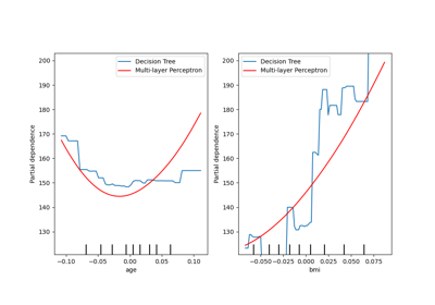
Partial Dependence and Individual Conditional Expectation Plots

Advanced Plotting With Partial Dependence

sklearn.neural_network.MLPRegressor¶

Examples using sklearn.neural_network.MLPRegressor¶

`sklearn.neural_network`.MLPRegressor¶

Examples using `sklearn.neural_network.MLPRegressor`¶