sklearn.inspection.plot_partial_dependence

sklearn.inspection.plot_partial_dependence(estimator, X, features, *, feature_names=None, target=None, response_method='auto', n_cols=3, grid_resolution=100, percentiles=(0.05, 0.95), method='auto', n_jobs=None, verbose=0, line_kw=None, ice_lines_kw=None, pd_line_kw=None, contour_kw=None, ax=None, kind='average', subsample=1000, random_state=None, centered=False)

DEPRECATED: Function plot_partial_dependence is deprecated in 1.0 and will be removed in 1.2. Use PartialDependenceDisplay.from_estimator instead

Partial dependence (PD) and individual conditional expectation (ICE) plots.

Partial dependence plots, individual conditional expectation plots or an overlay of both of them can be plotted by setting the kind parameter.

The ICE and PD plots can be centered with the parameter centered.

The len(features) plots are arranged in a grid with n_cols columns. Two-way partial dependence plots are plotted as contour plots. The deciles of the feature values will be shown with tick marks on the x-axes for one-way plots, and on both axes for two-way plots.

Read more in the User Guide.

Note

plot_partial_dependence does not support using the same axes with multiple calls. To plot the partial dependence for multiple estimators, please pass the axes created by the first call to the second call:

>>> from sklearn.inspection import plot_partial_dependence
>>> from sklearn.datasets import make_friedman1
>>> from sklearn.linear_model import LinearRegression
>>> from sklearn.ensemble import RandomForestRegressor
>>> X, y = make_friedman1()
>>> est1 = LinearRegression().fit(X, y)
>>> est2 = RandomForestRegressor().fit(X, y)
>>> disp1 = plot_partial_dependence(est1, X,
...                                 [1, 2])  
>>> disp2 = plot_partial_dependence(est2, X, [1, 2],
...                                 ax=disp1.axes_)  

Warning

For GradientBoostingClassifier and GradientBoostingRegressor, the 'recursion' method (used by default) will not account for the init predictor of the boosting process. In practice, this will produce the same values as 'brute' up to a constant offset in the target response, provided that init is a constant estimator (which is the default). However, if init is not a constant estimator, the partial dependence values are incorrect for 'recursion' because the offset will be sample-dependent. It is preferable to use the 'brute' method. Note that this only applies to GradientBoostingClassifier and GradientBoostingRegressor, not to HistGradientBoostingClassifier and HistGradientBoostingRegressor.

Deprecated since version 1.0: plot_partial_dependence is deprecated in 1.0 and will be removed in 1.2. Please use the class method: from_estimator.

Parameters:

estimatorBaseEstimator

A fitted estimator object implementing predict, predict_proba, or decision_function. Multioutput-multiclass classifiers are not supported.

X{array-like, dataframe} of shape (n_samples, n_features)

X is used to generate a grid of values for the target features (where the partial dependence will be evaluated), and also to generate values for the complement features when the method is 'brute'.

featureslist of {int, str, pair of int, pair of str}

The target features for which to create the PDPs. If features[i] is an integer or a string, a one-way PDP is created; if features[i] is a tuple, a two-way PDP is created (only supported with kind='average'). Each tuple must be of size 2. if any entry is a string, then it must be in feature_names.

feature_namesarray-like of shape (n_features,), dtype=str, default=None

Name of each feature; feature_names[i] holds the name of the feature with index i. By default, the name of the feature corresponds to their numerical index for NumPy array and their column name for pandas dataframe.

targetint, default=None

• In a multiclass setting, specifies the class for which the PDPs should be computed. Note that for binary classification, the positive class (index 1) is always used.

• In a multioutput setting, specifies the task for which the PDPs should be computed.

Ignored in binary classification or classical regression settings.

response_method{‘auto’, ‘predict_proba’, ‘decision_function’}, default=’auto’

Specifies whether to use predict_proba or decision_function as the target response. For regressors this parameter is ignored and the response is always the output of predict. By default, predict_proba is tried first and we revert to decision_function if it doesn’t exist. If method is 'recursion', the response is always the output of decision_function.

n_colsint, default=3

The maximum number of columns in the grid plot. Only active when ax is a single axis or None.

grid_resolutionint, default=100

The number of equally spaced points on the axes of the plots, for each target feature.

percentilestuple of float, default=(0.05, 0.95)

The lower and upper percentile used to create the extreme values for the PDP axes. Must be in [0, 1].

methodstr, default=’auto’

The method used to calculate the averaged predictions:

• 'recursion' is only supported for some tree-based estimators (namely GradientBoostingClassifier, GradientBoostingRegressor, HistGradientBoostingClassifier, HistGradientBoostingRegressor, DecisionTreeRegressor, RandomForestRegressor but is more efficient in terms of speed. With this method, the target response of a classifier is always the decision function, not the predicted probabilities. Since the 'recursion' method implicitly computes the average of the ICEs by design, it is not compatible with ICE and thus kind must be 'average'.

• 'brute' is supported for any estimator, but is more computationally intensive.

• 'auto': the 'recursion' is used for estimators that support it, and 'brute' is used otherwise.

Please see this note for differences between the 'brute' and 'recursion' method.

n_jobsint, default=None

The number of CPUs to use to compute the partial dependences. Computation is parallelized over features specified by the features parameter.

None means 1 unless in a joblib.parallel_backend context. -1 means using all processors. See Glossary for more details.

verboseint, default=0

Verbose output during PD computations.

line_kwdict, default=None

Dict with keywords passed to the matplotlib.pyplot.plot call. For one-way partial dependence plots. It can be used to define common properties for both ice_lines_kw and pdp_line_kw.

ice_lines_kwdict, default=None

Dictionary with keywords passed to the matplotlib.pyplot.plot call. For ICE lines in the one-way partial dependence plots. The key value pairs defined in ice_lines_kw takes priority over line_kw.

New in version 1.0.

pd_line_kwdict, default=None

Dictionary with keywords passed to the matplotlib.pyplot.plot call. For partial dependence in one-way partial dependence plots. The key value pairs defined in pd_line_kw takes priority over line_kw.

New in version 1.0.

contour_kwdict, default=None

Dict with keywords passed to the matplotlib.pyplot.contourf call. For two-way partial dependence plots.

axMatplotlib axes or array-like of Matplotlib axes, default=None

• If a single axis is passed in, it is treated as a bounding axes and a grid of partial dependence plots will be drawn within these bounds. The n_cols parameter controls the number of columns in the grid.

• If an array-like of axes are passed in, the partial dependence plots will be drawn directly into these axes.

• If None, a figure and a bounding axes is created and treated as the single axes case.

New in version 0.22.

kind{‘average’, ‘individual’, ‘both’} or list of such str, default=’average’

Whether to plot the partial dependence averaged across all the samples in the dataset or one line per sample or both.

• kind='average' results in the traditional PD plot;

• kind='individual' results in the ICE plot;

• kind='both' results in plotting both the ICE and PD on the same plot.

A list of such strings can be provided to specify kind on a per-plot basis. The length of the list should be the same as the number of interaction requested in features.

Note

ICE (‘individual’ or ‘both’) is not a valid option for 2-ways interactions plot. As a result, an error will be raised. 2-ways interaction plots should always be configured to use the ‘average’ kind instead.

Note

The fast method='recursion' option is only available for kind='average'. Plotting individual dependencies requires using the slower method='brute' option.

New in version 0.24: Add kind parameter with 'average', 'individual', and 'both' options.

New in version 1.1: Add the possibility to pass a list of string specifying kind for each plot.

subsamplefloat, int or None, default=1000

Sampling for ICE curves when kind is ‘individual’ or ‘both’. If float, should be between 0.0 and 1.0 and represent the proportion of the dataset to be used to plot ICE curves. If int, represents the absolute number samples to use.

Note that the full dataset is still used to calculate averaged partial dependence when kind='both'.

New in version 0.24.

random_stateint, RandomState instance or None, default=None

Controls the randomness of the selected samples when subsamples is not None and kind is either 'both' or 'individual'. See Glossary for details.

New in version 0.24.

centeredbool, default=False

If True, the ICE and PD lines will start at the origin of the y-axis. By default, no centering is done.

New in version 1.1.

Returns:

displayPartialDependenceDisplay

See also

partial_dependence

Compute Partial Dependence values.

PartialDependenceDisplay

Partial Dependence visualization.

PartialDependenceDisplay.from_estimator

Plot Partial Dependence.

Examples

>>> import matplotlib.pyplot as plt
>>> from sklearn.datasets import make_friedman1
>>> from sklearn.ensemble import GradientBoostingRegressor
>>> from sklearn.inspection import plot_partial_dependence
>>> X, y = make_friedman1()
>>> clf = GradientBoostingRegressor(n_estimators=10).fit(X, y)
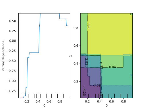
>>> plot_partial_dependence(clf, X, [0, (0, 1)])  
<...>
>>> plt.show()  

Examples using sklearn.inspection.plot_partial_dependence

Release Highlights for scikit-learn 0.24

Release Highlights for scikit-learn 0.24

Release Highlights for scikit-learn 0.23

Release Highlights for scikit-learn 0.23

Advanced Plotting With Partial Dependence

Advanced Plotting With Partial Dependence