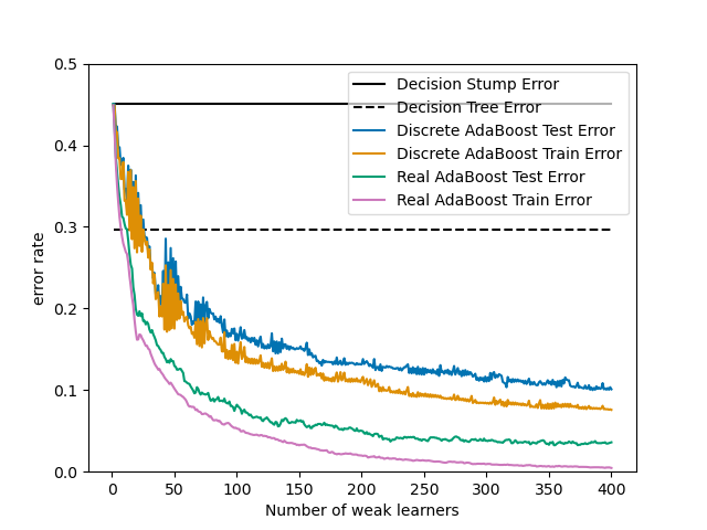
Discrete versus Real AdaBoost

This notebook is based on Figure 10.2 from Hastie et al 2009 [1] and illustrates the difference in performance between the discrete SAMME [2] boosting algorithm and real SAMME.R boosting algorithm. Both algorithms are evaluated on a binary classification task where the target Y is a non-linear function of 10 input features.

Discrete SAMME AdaBoost adapts based on errors in predicted class labels whereas real SAMME.R uses the predicted class probabilities.

[1]

T. Hastie, R. Tibshirani and J. Friedman, “Elements of Statistical Learning Ed. 2”, Springer, 2009.

[2]

J Zhu, H. Zou, S. Rosset, T. Hastie, “Multi-class AdaBoost”, Statistics and Its Interface, 2009.

Preparing the data and baseline models

We start by generating the binary classification dataset used in Hastie et al. 2009, Example 10.2.

# Authors: Peter Prettenhofer <peter.prettenhofer@gmail.com>,
#          Noel Dawe <noel.dawe@gmail.com>
#
# License: BSD 3 clause

from sklearn import datasets

X, y = datasets.make_hastie_10_2(n_samples=12_000, random_state=1)

Now, we set the hyperparameters for our AdaBoost classifiers. Be aware, a learning rate of 1.0 may not be optimal for both SAMME and SAMME.R

n_estimators = 400
learning_rate = 1.0

We split the data into a training and a test set. Then, we train our baseline classifiers, a DecisionTreeClassifier with depth=9 and a “stump” DecisionTreeClassifier with depth=1 and compute the test error.

from sklearn.model_selection import train_test_split
from sklearn.tree import DecisionTreeClassifier

X_train, X_test, y_train, y_test = train_test_split(
    X, y, test_size=2_000, shuffle=False
)

dt_stump = DecisionTreeClassifier(max_depth=1, min_samples_leaf=1)
dt_stump.fit(X_train, y_train)
dt_stump_err = 1.0 - dt_stump.score(X_test, y_test)

dt = DecisionTreeClassifier(max_depth=9, min_samples_leaf=1)
dt.fit(X_train, y_train)
dt_err = 1.0 - dt.score(X_test, y_test)

Adaboost with discrete SAMME and real SAMME.R

We now define the discrete and real AdaBoost classifiers and fit them to the training set.

from sklearn.ensemble import AdaBoostClassifier

ada_discrete = AdaBoostClassifier(
    base_estimator=dt_stump,
    learning_rate=learning_rate,
    n_estimators=n_estimators,
    algorithm="SAMME",
)
ada_discrete.fit(X_train, y_train)

AdaBoostClassifier(algorithm='SAMME',
                   base_estimator=DecisionTreeClassifier(max_depth=1),
                   n_estimators=400)

In a Jupyter environment, please rerun this cell to show the HTML representation or trust the notebook.
On GitHub, the HTML representation is unable to render, please try loading this page with nbviewer.org.

ada_real = AdaBoostClassifier(
    base_estimator=dt_stump,
    learning_rate=learning_rate,
    n_estimators=n_estimators,
    algorithm="SAMME.R",
)
ada_real.fit(X_train, y_train)

AdaBoostClassifier(base_estimator=DecisionTreeClassifier(max_depth=1),
                   n_estimators=400)

In a Jupyter environment, please rerun this cell to show the HTML representation or trust the notebook.
On GitHub, the HTML representation is unable to render, please try loading this page with nbviewer.org.

Now, let’s compute the test error of the discrete and real AdaBoost classifiers for each new stump in n_estimators added to the ensemble.

import numpy as np
from sklearn.metrics import zero_one_loss

ada_discrete_err = np.zeros((n_estimators,))
for i, y_pred in enumerate(ada_discrete.staged_predict(X_test)):
    ada_discrete_err[i] = zero_one_loss(y_pred, y_test)

ada_discrete_err_train = np.zeros((n_estimators,))
for i, y_pred in enumerate(ada_discrete.staged_predict(X_train)):
    ada_discrete_err_train[i] = zero_one_loss(y_pred, y_train)

ada_real_err = np.zeros((n_estimators,))
for i, y_pred in enumerate(ada_real.staged_predict(X_test)):
    ada_real_err[i] = zero_one_loss(y_pred, y_test)

ada_real_err_train = np.zeros((n_estimators,))
for i, y_pred in enumerate(ada_real.staged_predict(X_train)):
    ada_real_err_train[i] = zero_one_loss(y_pred, y_train)

Plotting the results

Finally, we plot the train and test errors of our baselines and of the discrete and real AdaBoost classifiers

import matplotlib.pyplot as plt
import seaborn as sns

fig = plt.figure()
ax = fig.add_subplot(111)

ax.plot([1, n_estimators], [dt_stump_err] * 2, "k-", label="Decision Stump Error")
ax.plot([1, n_estimators], [dt_err] * 2, "k--", label="Decision Tree Error")

colors = sns.color_palette("colorblind")

ax.plot(
    np.arange(n_estimators) + 1,
    ada_discrete_err,
    label="Discrete AdaBoost Test Error",
    color=colors[0],
)
ax.plot(
    np.arange(n_estimators) + 1,
    ada_discrete_err_train,
    label="Discrete AdaBoost Train Error",
    color=colors[1],
)
ax.plot(
    np.arange(n_estimators) + 1,
    ada_real_err,
    label="Real AdaBoost Test Error",
    color=colors[2],
)
ax.plot(
    np.arange(n_estimators) + 1,
    ada_real_err_train,
    label="Real AdaBoost Train Error",
    color=colors[4],
)

ax.set_ylim((0.0, 0.5))
ax.set_xlabel("Number of weak learners")
ax.set_ylabel("error rate")

leg = ax.legend(loc="upper right", fancybox=True)
leg.get_frame().set_alpha(0.7)

plt.show()

Concluding remarks

We observe that the error rate for both train and test sets of real AdaBoost is lower than that of discrete AdaBoost.