Note
Click here to download the full example code or to run this example in your browser via Binder
Isotonic Regression
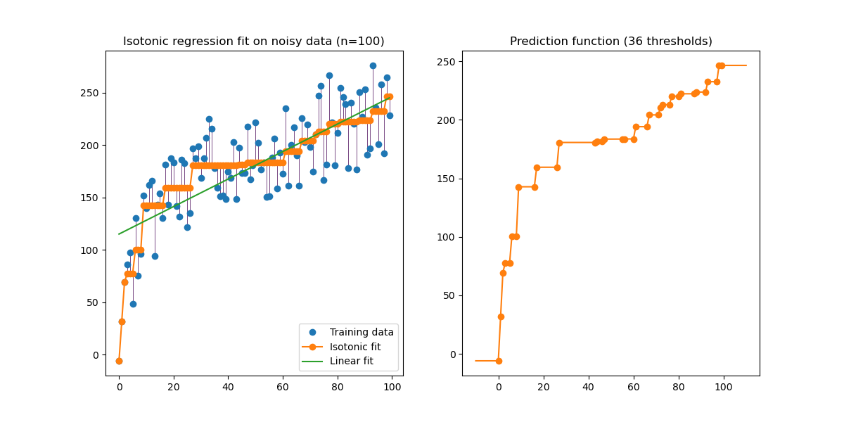
An illustration of the isotonic regression on generated data (non-linear monotonic trend with homoscedastic uniform noise).
The isotonic regression algorithm finds a non-decreasing approximation of a function while minimizing the mean squared error on the training data. The benefit of such a non-parametric model is that it does not assume any shape for the target function besides monotonicity. For comparison a linear regression is also presented.
The plot on the right-hand side shows the model prediction function that results from the linear interpolation of thresholds points. The thresholds points are a subset of the training input observations and their matching target values are computed by the isotonic non-parametric fit.
# Author: Nelle Varoquaux <nelle.varoquaux@gmail.com>
#         Alexandre Gramfort <alexandre.gramfort@inria.fr>
# License: BSD

import numpy as np
import matplotlib.pyplot as plt
from matplotlib.collections import LineCollection

from sklearn.linear_model import LinearRegression
from sklearn.isotonic import IsotonicRegression
from sklearn.utils import check_random_state

n = 100
x = np.arange(n)
rs = check_random_state(0)
y = rs.randint(-50, 50, size=(n,)) + 50.0 * np.log1p(np.arange(n))
Fit IsotonicRegression and LinearRegression models:
ir = IsotonicRegression(out_of_bounds="clip")
y_ = ir.fit_transform(x, y)

lr = LinearRegression()
lr.fit(x[:, np.newaxis], y)  # x needs to be 2d for LinearRegression
Plot results:
segments = [[[i, y[i]], [i, y_[i]]] for i in range(n)]
lc = LineCollection(segments, zorder=0)
lc.set_array(np.ones(len(y)))
lc.set_linewidths(np.full(n, 0.5))

fig, (ax0, ax1) = plt.subplots(ncols=2, figsize=(12, 6))

ax0.plot(x, y, "C0.", markersize=12)
ax0.plot(x, y_, "C1.-", markersize=12)
ax0.plot(x, lr.predict(x[:, np.newaxis]), "C2-")
ax0.add_collection(lc)
ax0.legend(("Training data", "Isotonic fit", "Linear fit"), loc="lower right")
ax0.set_title("Isotonic regression fit on noisy data (n=%d)" % n)

x_test = np.linspace(-10, 110, 1000)
ax1.plot(x_test, ir.predict(x_test), "C1-")
ax1.plot(ir.X_thresholds_, ir.y_thresholds_, "C1.", markersize=12)
ax1.set_title("Prediction function (%d thresholds)" % len(ir.X_thresholds_))

plt.show()
Note that we explicitly passed out_of_bounds="clip" to the constructor of
IsotonicRegression to control the way the model extrapolates outside of the
range of data observed in the training set. This “clipping” extrapolation can
be seen on the plot of the decision function on the right-hand.
Total running time of the script: ( 0 minutes 0.124 seconds)