1.16. Probability calibration
When performing classification you often want not only to predict the class
label, but also obtain a probability of the respective label. This probability
gives you some kind of confidence on the prediction. Some models can give you
poor estimates of the class probabilities and some even do not support
probability prediction (e.g., some instances of
SGDClassifier).
The calibration module allows you to better calibrate
the probabilities of a given model, or to add support for probability
prediction.
Well calibrated classifiers are probabilistic classifiers for which the output of the predict_proba method can be directly interpreted as a confidence level. For instance, a well calibrated (binary) classifier should classify the samples such that among the samples to which it gave a predict_proba value close to 0.8, approximately 80% actually belong to the positive class.
1.16.1. Calibration curves
The following plot compares how well the probabilistic predictions of
different classifiers are calibrated, using calibration_curve.
The x axis represents the average predicted probability in each bin. The
y axis is the fraction of positives, i.e. the proportion of samples whose
class is the positive class (in each bin).
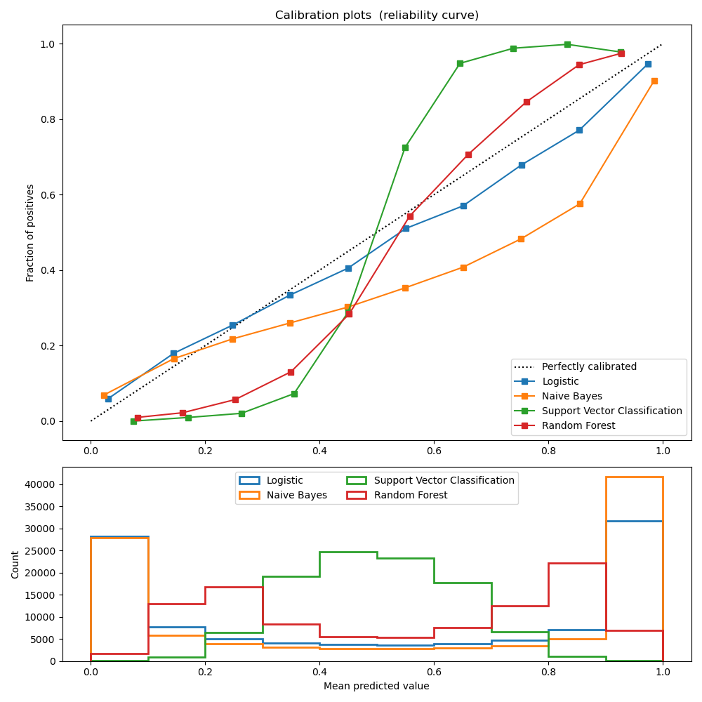
LogisticRegression returns well calibrated predictions by default as it directly
optimizes Log loss. In contrast, the other methods return biased probabilities;
with different biases per method:
GaussianNB tends to push probabilities to 0 or 1 (note the counts
in the histograms). This is mainly because it makes the assumption that
features are conditionally independent given the class, which is not the
case in this dataset which contains 2 redundant features.
RandomForestClassifier shows the opposite behavior: the histograms
show peaks at approximately 0.2 and 0.9 probability, while probabilities
close to 0 or 1 are very rare. An explanation for this is given by
Niculescu-Mizil and Caruana 1: “Methods such as bagging and random
forests that average predictions from a base set of models can have
difficulty making predictions near 0 and 1 because variance in the
underlying base models will bias predictions that should be near zero or one
away from these values. Because predictions are restricted to the interval
[0,1], errors caused by variance tend to be one-sided near zero and one. For
example, if a model should predict p = 0 for a case, the only way bagging
can achieve this is if all bagged trees predict zero. If we add noise to the
trees that bagging is averaging over, this noise will cause some trees to
predict values larger than 0 for this case, thus moving the average
prediction of the bagged ensemble away from 0. We observe this effect most
strongly with random forests because the base-level trees trained with
random forests have relatively high variance due to feature subsetting.” As
a result, the calibration curve also referred to as the reliability diagram
(Wilks 1995 2) shows a characteristic sigmoid shape, indicating that the
classifier could trust its “intuition” more and return probabilities closer
to 0 or 1 typically.
Linear Support Vector Classification (LinearSVC) shows an even more
sigmoid curve than RandomForestClassifier, which is
typical for maximum-margin methods (compare Niculescu-Mizil and Caruana 1),
which focus on difficult to classify samples that are close to the decision
boundary (the support vectors).
1.16.2. Calibrating a classifier
Calibrating a classifier consists of fitting a regressor (called a calibrator) that maps the output of the classifier (as given by decision_function or predict_proba) to a calibrated probability in [0, 1]. Denoting the output of the classifier for a given sample by \(f_i\), the calibrator tries to predict \(p(y_i = 1 | f_i)\).
The samples that are used to fit the calibrator should not be the same samples used to fit the classifier, as this would introduce bias. This is because performance of the classifier on its training data would be better than for novel data. Using the classifier output of training data to fit the calibrator would thus result in a biased calibrator that maps to probabilities closer to 0 and 1 than it should.
1.16.3. Usage
The CalibratedClassifierCV class is used to calibrate a classifier.
CalibratedClassifierCV uses a cross-validation approach to ensure
unbiased data is always used to fit the calibrator. The data is split into k
(train_set, test_set) couples (as determined by cv). When ensemble=True
(default), the following procedure is repeated independently for each
cross-validation split: a clone of base_estimator is first trained on the
train subset. Then its predictions on the test subset are used to fit a
calibrator (either a sigmoid or isotonic regressor). This results in an
ensemble of k (classifier, calibrator) couples where each calibrator maps
the output of its corresponding classifier into [0, 1]. Each couple is exposed
in the calibrated_classifiers_ attribute, where each entry is a calibrated
classifier with a predict_proba method that outputs calibrated
probabilities. The output of predict_proba for the main
CalibratedClassifierCV instance corresponds to the average of the
predicted probabilities of the k estimators in the calibrated_classifiers_
list. The output of predict is the class that has the highest
probability.
When ensemble=False, cross-validation is used to obtain ‘unbiased’
predictions for all the data, via
cross_val_predict.
These unbiased predictions are then used to train the calibrator. The attribute
calibrated_classifiers_ consists of only one (classifier, calibrator)
couple where the classifier is the base_estimator trained on all the data.
In this case the output of predict_proba for
CalibratedClassifierCV is the predicted probabilities obtained
from the single (classifier, calibrator) couple.
The main advantage of ensemble=True is to benefit from the traditional
ensembling effect (similar to Bagging meta-estimator). The resulting ensemble should
both be well calibrated and slightly more accurate than with ensemble=False.
The main advantage of using ensemble=False is computational: it reduces the
overall fit time by training only a single base classifier and calibrator
pair, decreases the final model size and increases prediction speed.
Alternatively an already fitted classifier can be calibrated by setting
cv="prefit". In this case, the data is not split and all of it is used to
fit the regressor. It is up to the user to
make sure that the data used for fitting the classifier is disjoint from the
data used for fitting the regressor.
sklearn.metrics.brier_score_loss may be used to assess how
well a classifier is calibrated. However, this metric should be used with care
because a lower Brier score does not always mean a better calibrated model.
This is because the Brier score metric is a combination of calibration loss
and refinement loss. Calibration loss is defined as the mean squared deviation
from empirical probabilities derived from the slope of ROC segments.
Refinement loss can be defined as the expected optimal loss as measured by the
area under the optimal cost curve. As refinement loss can change
independently from calibration loss, a lower Brier score does not necessarily
mean a better calibrated model.
CalibratedClassifierCV supports the use of two ‘calibration’
regressors: ‘sigmoid’ and ‘isotonic’.
1.16.3.1. Sigmoid
The sigmoid regressor is based on Platt’s logistic model 3:
where \(y_i\) is the true label of sample \(i\) and \(f_i\) is the output of the un-calibrated classifier for sample \(i\). \(A\) and \(B\) are real numbers to be determined when fitting the regressor via maximum likelihood.
The sigmoid method assumes the calibration curve can be corrected by applying a sigmoid function to the raw predictions. This assumption has been empirically justified in the case of Support Vector Machines with common kernel functions on various benchmark datasets in section 2.1 of Platt 1999 3 but does not necessarily hold in general. Additionally, the logistic model works best if the calibration error is symmetrical, meaning the classifier output for each binary class is normally distributed with the same variance 6. This can be a problem for highly imbalanced classification problems, where outputs do not have equal variance.
In general this method is most effective when the un-calibrated model is under-confident and has similar calibration errors for both high and low outputs.
1.16.3.2. Isotonic
The ‘isotonic’ method fits a non-parametric isotonic regressor, which outputs
a step-wise non-decreasing function (see sklearn.isotonic). It
minimizes:
subject to \(\hat{f}_i >= \hat{f}_j\) whenever \(f_i >= f_j\). \(y_i\) is the true label of sample \(i\) and \(\hat{f}_i\) is the output of the calibrated classifier for sample \(i\) (i.e., the calibrated probability). This method is more general when compared to ‘sigmoid’ as the only restriction is that the mapping function is monotonically increasing. It is thus more powerful as it can correct any monotonic distortion of the un-calibrated model. However, it is more prone to overfitting, especially on small datasets 5.
Overall, ‘isotonic’ will perform as well as or better than ‘sigmoid’ when there is enough data (greater than ~ 1000 samples) to avoid overfitting 1.
1.16.3.3. Multiclass support
Both isotonic and sigmoid regressors only
support 1-dimensional data (e.g., binary classification output) but are
extended for multiclass classification if the base_estimator supports
multiclass predictions. For multiclass predictions,
CalibratedClassifierCV calibrates for
each class separately in a OneVsRestClassifier fashion 4. When
predicting
probabilities, the calibrated probabilities for each class
are predicted separately. As those probabilities do not necessarily sum to
one, a postprocessing is performed to normalize them.
Examples:
References:
- 1(1,2,3)
Predicting Good Probabilities with Supervised Learning, A. Niculescu-Mizil & R. Caruana, ICML 2005
- 2
On the combination of forecast probabilities for consecutive precipitation periods. Wea. Forecasting, 5, 640–650., Wilks, D. S., 1990a
- 3(1,2)
Probabilistic Outputs for Support Vector Machines and Comparisons to Regularized Likelihood Methods. J. Platt, (1999)
- 4
Transforming Classifier Scores into Accurate Multiclass Probability Estimates. B. Zadrozny & C. Elkan, (KDD 2002)
- 5
Predicting accurate probabilities with a ranking loss. Menon AK, Jiang XJ, Vembu S, Elkan C, Ohno-Machado L. Proc Int Conf Mach Learn. 2012;2012:703-710
- 6
Beyond sigmoids: How to obtain well-calibrated probabilities from binary classifiers with beta calibration Kull, M., Silva Filho, T. M., & Flach, P. (2017).