Note
Click here to download the full example code or to run this example in your browser via Binder
Imputing missing values with variants of IterativeImputer
The IterativeImputer class is very flexible - it can be
used with a variety of estimators to do round-robin regression, treating every
variable as an output in turn.
In this example we compare some estimators for the purpose of missing feature
imputation with IterativeImputer:
BayesianRidge: regularized linear regressionDecisionTreeRegressor: non-linear regressionExtraTreesRegressor: similar to missForest in RKNeighborsRegressor: comparable to other KNN imputation approaches
Of particular interest is the ability of
IterativeImputer to mimic the behavior of missForest, a
popular imputation package for R. In this example, we have chosen to use
ExtraTreesRegressor instead of
RandomForestRegressor (as in missForest) due to its
increased speed.
Note that KNeighborsRegressor is different from KNN
imputation, which learns from samples with missing values by using a distance
metric that accounts for missing values, rather than imputing them.
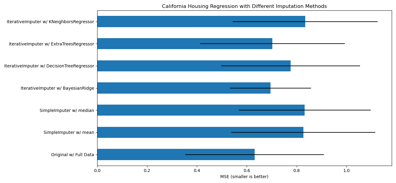
The goal is to compare different estimators to see which one is best for the
IterativeImputer when using a
BayesianRidge estimator on the California housing
dataset with a single value randomly removed from each row.
For this particular pattern of missing values we see that
ExtraTreesRegressor and
BayesianRidge give the best results.
print(__doc__)

import numpy as np
import matplotlib.pyplot as plt
import pandas as pd

# To use this experimental feature, we need to explicitly ask for it:
from sklearn.experimental import enable_iterative_imputer  # noqa
from sklearn.datasets import fetch_california_housing
from sklearn.impute import SimpleImputer
from sklearn.impute import IterativeImputer
from sklearn.linear_model import BayesianRidge
from sklearn.tree import DecisionTreeRegressor
from sklearn.ensemble import ExtraTreesRegressor
from sklearn.neighbors import KNeighborsRegressor
from sklearn.pipeline import make_pipeline
from sklearn.model_selection import cross_val_score

N_SPLITS = 5

rng = np.random.RandomState(0)

X_full, y_full = fetch_california_housing(return_X_y=True)
# ~2k samples is enough for the purpose of the example.
# Remove the following two lines for a slower run with different error bars.
X_full = X_full[::10]
y_full = y_full[::10]
n_samples, n_features = X_full.shape

# Estimate the score on the entire dataset, with no missing values
br_estimator = BayesianRidge()
score_full_data = pd.DataFrame(
    cross_val_score(
        br_estimator, X_full, y_full, scoring='neg_mean_squared_error',
        cv=N_SPLITS
    ),
    columns=['Full Data']
)

# Add a single missing value to each row
X_missing = X_full.copy()
y_missing = y_full
missing_samples = np.arange(n_samples)
missing_features = rng.choice(n_features, n_samples, replace=True)
X_missing[missing_samples, missing_features] = np.nan

# Estimate the score after imputation (mean and median strategies)
score_simple_imputer = pd.DataFrame()
for strategy in ('mean', 'median'):
    estimator = make_pipeline(
        SimpleImputer(missing_values=np.nan, strategy=strategy),
        br_estimator
    )
    score_simple_imputer[strategy] = cross_val_score(
        estimator, X_missing, y_missing, scoring='neg_mean_squared_error',
        cv=N_SPLITS
    )

# Estimate the score after iterative imputation of the missing values
# with different estimators
estimators = [
    BayesianRidge(),
    DecisionTreeRegressor(max_features='sqrt', random_state=0),
    ExtraTreesRegressor(n_estimators=10, random_state=0),
    KNeighborsRegressor(n_neighbors=15)
]
score_iterative_imputer = pd.DataFrame()
for impute_estimator in estimators:
    estimator = make_pipeline(
        IterativeImputer(random_state=0, estimator=impute_estimator),
        br_estimator
    )
    score_iterative_imputer[impute_estimator.__class__.__name__] = \
        cross_val_score(
            estimator, X_missing, y_missing, scoring='neg_mean_squared_error',
            cv=N_SPLITS
        )

scores = pd.concat(
    [score_full_data, score_simple_imputer, score_iterative_imputer],
    keys=['Original', 'SimpleImputer', 'IterativeImputer'], axis=1
)

# plot california housing results
fig, ax = plt.subplots(figsize=(13, 6))
means = -scores.mean()
errors = scores.std()
means.plot.barh(xerr=errors, ax=ax)
ax.set_title('California Housing Regression with Different Imputation Methods')
ax.set_xlabel('MSE (smaller is better)')
ax.set_yticks(np.arange(means.shape[0]))
ax.set_yticklabels([" w/ ".join(label) for label in means.index.tolist()])
plt.tight_layout(pad=1)
plt.show()
Total running time of the script: ( 0 minutes 24.052 seconds)