Note
Click here to download the full example code or to run this example in your browser via Binder
SVM Exercise
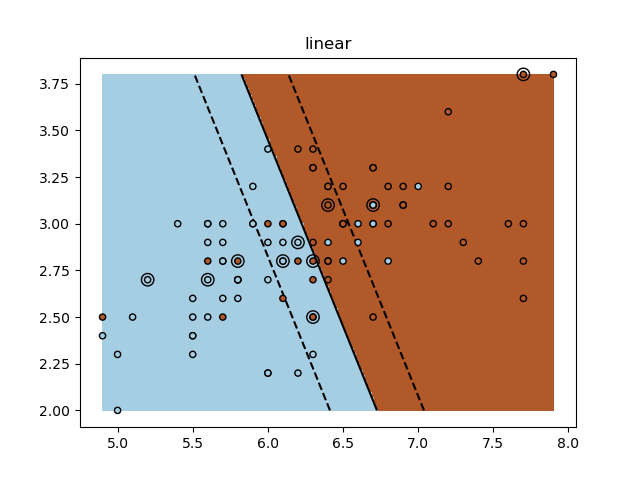
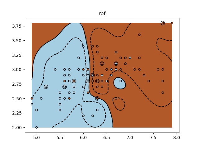
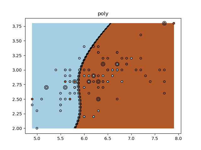
A tutorial exercise for using different SVM kernels.
This exercise is used in the Using kernels part of the Supervised learning: predicting an output variable from high-dimensional observations section of the A tutorial on statistical-learning for scientific data processing.
Out:
/home/circleci/project/examples/exercises/plot_iris_exercise.py:62: MatplotlibDeprecationWarning: shading='flat' when X and Y have the same dimensions as C is deprecated since 3.3. Either specify the corners of the quadrilaterals with X and Y, or pass shading='auto', 'nearest' or 'gouraud', or set rcParams['pcolor.shading']. This will become an error two minor releases later.
plt.pcolormesh(XX, YY, Z > 0, cmap=plt.cm.Paired)
print(__doc__)


import numpy as np
import matplotlib.pyplot as plt
from sklearn import datasets, svm

iris = datasets.load_iris()
X = iris.data
y = iris.target

X = X[y != 0, :2]
y = y[y != 0]

n_sample = len(X)

np.random.seed(0)
order = np.random.permutation(n_sample)
X = X[order]
y = y[order].astype(float)

X_train = X[:int(.9 * n_sample)]
y_train = y[:int(.9 * n_sample)]
X_test = X[int(.9 * n_sample):]
y_test = y[int(.9 * n_sample):]

# fit the model
for kernel in ('linear', 'rbf', 'poly'):
    clf = svm.SVC(kernel=kernel, gamma=10)
    clf.fit(X_train, y_train)

    plt.figure()
    plt.clf()
    plt.scatter(X[:, 0], X[:, 1], c=y, zorder=10, cmap=plt.cm.Paired,
                edgecolor='k', s=20)

    # Circle out the test data
    plt.scatter(X_test[:, 0], X_test[:, 1], s=80, facecolors='none',
                zorder=10, edgecolor='k')

    plt.axis('tight')
    x_min = X[:, 0].min()
    x_max = X[:, 0].max()
    y_min = X[:, 1].min()
    y_max = X[:, 1].max()

    XX, YY = np.mgrid[x_min:x_max:200j, y_min:y_max:200j]
    Z = clf.decision_function(np.c_[XX.ravel(), YY.ravel()])

    # Put the result into a color plot
    Z = Z.reshape(XX.shape)
    plt.pcolormesh(XX, YY, Z > 0, cmap=plt.cm.Paired)
    plt.contour(XX, YY, Z, colors=['k', 'k', 'k'],
                linestyles=['--', '-', '--'], levels=[-.5, 0, .5])

    plt.title(kernel)
plt.show()
Total running time of the script: ( 0 minutes 7.148 seconds)


