Note
Click here to download the full example code or to run this example in your browser via Binder
Monotonic Constraints
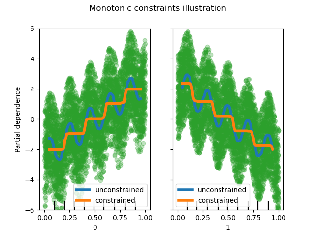
This example illustrates the effect of monotonic constraints on a gradient boosting estimator.
We build an artificial dataset where the target value is in general positively correlated with the first feature (with some random and non-random variations), and in general negatively correlated with the second feature.
By imposing a positive (increasing) or negative (decreasing) constraint on the features during the learning process, the estimator is able to properly follow the general trend instead of being subject to the variations.
This example was inspired by the XGBoost documentation.
from sklearn.experimental import enable_hist_gradient_boosting  # noqa
from sklearn.ensemble import HistGradientBoostingRegressor
from sklearn.inspection import plot_partial_dependence
import numpy as np
import matplotlib.pyplot as plt


print(__doc__)

rng = np.random.RandomState(0)

n_samples = 5000
f_0 = rng.rand(n_samples)  # positive correlation with y
f_1 = rng.rand(n_samples)  # negative correlation with y
X = np.c_[f_0, f_1]
noise = rng.normal(loc=0.0, scale=0.01, size=n_samples)
y = (5 * f_0 + np.sin(10 * np.pi * f_0) -
     5 * f_1 - np.cos(10 * np.pi * f_1) +
     noise)

fig, ax = plt.subplots()


# Without any constraint
gbdt = HistGradientBoostingRegressor()
gbdt.fit(X, y)
disp = plot_partial_dependence(
    gbdt,
    X,
    features=[0, 1],
    line_kw={"linewidth": 4, "label": "unconstrained", "color": "tab:blue"},
    ax=ax,
)

# With positive and negative constraints
gbdt = HistGradientBoostingRegressor(monotonic_cst=[1, -1])
gbdt.fit(X, y)

plot_partial_dependence(
    gbdt,
    X,
    features=[0, 1],
    feature_names=(
        "First feature\nPositive constraint",
        "Second feature\nNegtive constraint",
    ),
    line_kw={"linewidth": 4, "label": "constrained", "color": "tab:orange"},
    ax=disp.axes_,
)

for f_idx in (0, 1):
    disp.axes_[0, f_idx].plot(
        X[:, f_idx], y, "o", alpha=0.3, zorder=-1, color="tab:green"
    )
    disp.axes_[0, f_idx].set_ylim(-6, 6)

plt.legend()
fig.suptitle("Monotonic constraints illustration")

plt.show()
Total running time of the script: ( 0 minutes 0.848 seconds)