Note
Click here to download the full example code or to run this example in your browser via Binder
Gradient Boosting regression
This example demonstrates Gradient Boosting to produce a predictive
model from an ensemble of weak predictive models. Gradient boosting can be used
for regression and classification problems. Here, we will train a model to
tackle a diabetes regression task. We will obtain the results from
GradientBoostingRegressor with least squares loss
and 500 regression trees of depth 4.
Note: For larger datasets (n_samples >= 10000), please refer to
HistGradientBoostingRegressor.
print(__doc__)

# Author: Peter Prettenhofer <peter.prettenhofer@gmail.com>
#         Maria Telenczuk <https://github.com/maikia>
#         Katrina Ni <https://github.com/nilichen>
#
# License: BSD 3 clause

import matplotlib.pyplot as plt
import numpy as np
from sklearn import datasets, ensemble
from sklearn.inspection import permutation_importance
from sklearn.metrics import mean_squared_error
from sklearn.model_selection import train_test_split
Load the data
First we need to load the data.
diabetes = datasets.load_diabetes()
X, y = diabetes.data, diabetes.target
Data preprocessing
Next, we will split our dataset to use 90% for training and leave the rest for testing. We will also set the regression model parameters. You can play with these parameters to see how the results change.
n_estimators : the number of boosting stages that will be performed. Later, we will plot deviance against boosting iterations.
max_depth : limits the number of nodes in the tree. The best value depends on the interaction of the input variables.
min_samples_split : the minimum number of samples required to split an internal node.
learning_rate : how much the contribution of each tree will shrink.
loss : loss function to optimize. The least squares function is used in this
case however, there are many other options (see
GradientBoostingRegressor ).
X_train, X_test, y_train, y_test = train_test_split(
    X, y, test_size=0.1, random_state=13)

params = {'n_estimators': 500,
          'max_depth': 4,
          'min_samples_split': 5,
          'learning_rate': 0.01,
          'loss': 'ls'}
Fit regression model
Now we will initiate the gradient boosting regressors and fit it with our training data. Let’s also look and the mean squared error on the test data.
reg = ensemble.GradientBoostingRegressor(**params)
reg.fit(X_train, y_train)

mse = mean_squared_error(y_test, reg.predict(X_test))
print("The mean squared error (MSE) on test set: {:.4f}".format(mse))
Out:
The mean squared error (MSE) on test set: 3017.9419
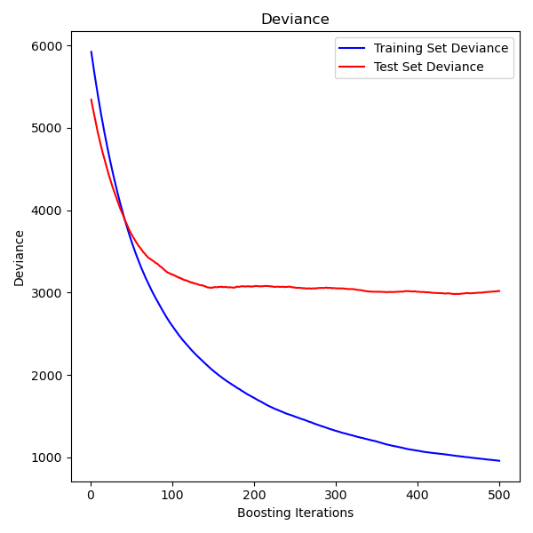
Plot training deviance
Finally, we will visualize the results. To do that we will first compute the test set deviance and then plot it against boosting iterations.
test_score = np.zeros((params['n_estimators'],), dtype=np.float64)
for i, y_pred in enumerate(reg.staged_predict(X_test)):
    test_score[i] = reg.loss_(y_test, y_pred)

fig = plt.figure(figsize=(6, 6))
plt.subplot(1, 1, 1)
plt.title('Deviance')
plt.plot(np.arange(params['n_estimators']) + 1, reg.train_score_, 'b-',
         label='Training Set Deviance')
plt.plot(np.arange(params['n_estimators']) + 1, test_score, 'r-',
         label='Test Set Deviance')
plt.legend(loc='upper right')
plt.xlabel('Boosting Iterations')
plt.ylabel('Deviance')
fig.tight_layout()
plt.show()
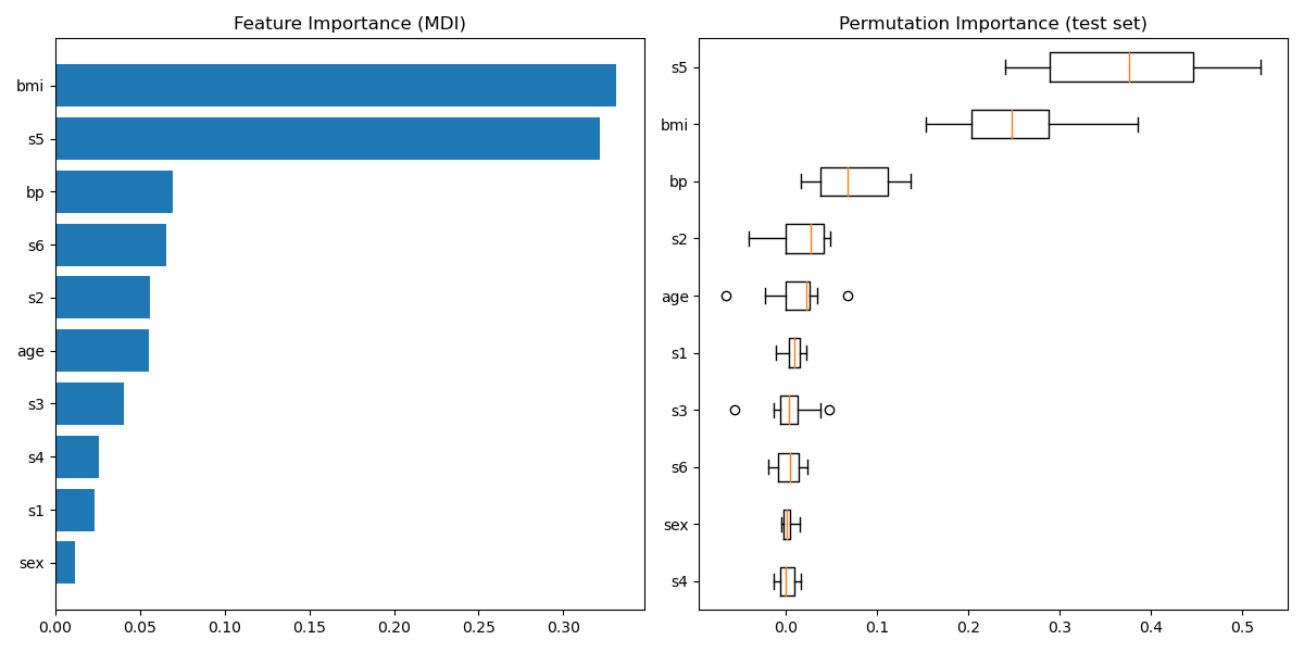
Plot feature importance
Careful, impurity-based feature importances can be misleading for
high cardinality features (many unique values). As an alternative,
the permutation importances of reg can be computed on a
held out test set. See Permutation feature importance for more details.
For this example, the impurity-based and permutation methods identify the same 2 strongly predictive features but not in the same order. The third most predictive feature, “bp”, is also the same for the 2 methods. The remaining features are less predictive and the error bars of the permutation plot show that they overlap with 0.
feature_importance = reg.feature_importances_
sorted_idx = np.argsort(feature_importance)
pos = np.arange(sorted_idx.shape[0]) + .5
fig = plt.figure(figsize=(12, 6))
plt.subplot(1, 2, 1)
plt.barh(pos, feature_importance[sorted_idx], align='center')
plt.yticks(pos, np.array(diabetes.feature_names)[sorted_idx])
plt.title('Feature Importance (MDI)')

result = permutation_importance(reg, X_test, y_test, n_repeats=10,
                                random_state=42, n_jobs=2)
sorted_idx = result.importances_mean.argsort()
plt.subplot(1, 2, 2)
plt.boxplot(result.importances[sorted_idx].T,
            vert=False, labels=np.array(diabetes.feature_names)[sorted_idx])
plt.title("Permutation Importance (test set)")
fig.tight_layout()
plt.show()
Total running time of the script: ( 0 minutes 1.243 seconds)