Categorical Feature Support in Gradient Boosting¶

Load Ames Housing dataset¶

First, we load the ames housing data as a pandas dataframe. The features are either categorical or numerical:

from sklearn.datasets import fetch_openml

X, y = fetch_openml(data_id=41211, as_frame=True, return_X_y=True)

n_categorical_features = (X.dtypes == 'category').sum()
n_numerical_features = (X.dtypes == 'float').sum()
print(f"Number of samples: {X.shape[0]}")
print(f"Number of features: {X.shape[1]}")
print(f"Number of categorical features: {n_categorical_features}")
print(f"Number of numerical features: {n_numerical_features}")

Out:

/home/circleci/project/sklearn/datasets/_openml.py:849: UserWarning: Version 1 of dataset ames-housing is inactive, meaning that issues have been found in the dataset. Try using a newer version from this URL: https://www.openml.org/data/v1/download/20649135/ames-housing.arff
  warn("Version {} of dataset {} is inactive, meaning that issues have "
Number of samples: 2930
Number of features: 80
Number of categorical features: 46
Number of numerical features: 34

Gradient boosting estimator with dropped categorical features¶

As a baseline, we create an estimator where the categorical features are dropped:

from sklearn.experimental import enable_hist_gradient_boosting  # noqa
from sklearn.ensemble import HistGradientBoostingRegressor
from sklearn.pipeline import make_pipeline
from sklearn.compose import make_column_transformer
from sklearn.compose import make_column_selector

dropper = make_column_transformer(
    ('drop', make_column_selector(dtype_include='category')),
    remainder='passthrough')
hist_dropped = make_pipeline(dropper,
                             HistGradientBoostingRegressor(random_state=42))

Gradient boosting estimator with one-hot encoding¶

Next, we create a pipeline that will one-hot encode the categorical features and let the rest of the numerical data to passthrough:

from sklearn.preprocessing import OneHotEncoder

one_hot_encoder = make_column_transformer(
    (OneHotEncoder(sparse=False, handle_unknown='ignore'),
     make_column_selector(dtype_include='category')),
    remainder='passthrough')

hist_one_hot = make_pipeline(one_hot_encoder,
                             HistGradientBoostingRegressor(random_state=42))

Gradient boosting estimator with ordinal encoding¶

Next, we create a pipeline that will treat categorical features as if they were ordered quantities, i.e. the categories will be encoded as 0, 1, 2, etc., and treated as continuous features.

from sklearn.preprocessing import OrdinalEncoder
import numpy as np

ordinal_encoder = make_column_transformer(
    (OrdinalEncoder(handle_unknown='use_encoded_value', unknown_value=np.nan),
     make_column_selector(dtype_include='category')),
    remainder='passthrough')

hist_ordinal = make_pipeline(ordinal_encoder,
                             HistGradientBoostingRegressor(random_state=42))

Gradient boosting estimator with native categorical support¶

We now create a HistGradientBoostingRegressor estimator that will natively handle categorical features. This estimator will not treat categorical features as ordered quantities.

Since the HistGradientBoostingRegressor requires category values to be encoded in [0, n_unique_categories - 1], we still rely on an OrdinalEncoder to pre-process the data.

The main difference between this pipeline and the previous one is that in this one, we let the HistGradientBoostingRegressor know which features are categorical.

# The ordinal encoder will first output the categorical features, and then the
# continuous (passed-through) features
categorical_mask = ([True] * n_categorical_features +
                    [False] * n_numerical_features)
hist_native = make_pipeline(
    ordinal_encoder,
    HistGradientBoostingRegressor(random_state=42,
                                  categorical_features=categorical_mask)
)

Model comparison¶

Finally, we evaluate the models using cross validation. Here we compare the models performance in terms of mean_absolute_percentage_error and fit times.

from sklearn.model_selection import cross_validate
import matplotlib.pyplot as plt

scoring = "neg_mean_absolute_percentage_error"
dropped_result = cross_validate(hist_dropped, X, y, cv=3, scoring=scoring)
one_hot_result = cross_validate(hist_one_hot, X, y, cv=3, scoring=scoring)
ordinal_result = cross_validate(hist_ordinal, X, y, cv=3, scoring=scoring)
native_result = cross_validate(hist_native, X, y, cv=3, scoring=scoring)


def plot_results(figure_title):
    fig, (ax1, ax2) = plt.subplots(1, 2, figsize=(12, 8))

    plot_info = [('fit_time', 'Fit times (s)', ax1, None),
                 ('test_score', 'Mean Absolute Percentage Error', ax2,
                  (0, 0.20))]

    x, width = np.arange(4), 0.9
    for key, title, ax, y_limit in plot_info:
        items = [dropped_result[key], one_hot_result[key], ordinal_result[key],
                 native_result[key]]
        ax.bar(x, [np.mean(np.abs(item)) for item in items],
               width, yerr=[np.std(item) for item in items],
               color=['C0', 'C1', 'C2', 'C3'])
        ax.set(xlabel='Model', title=title, xticks=x,
               xticklabels=["Dropped", "One Hot", "Ordinal", "Native"],
               ylim=y_limit)
    fig.suptitle(figure_title)


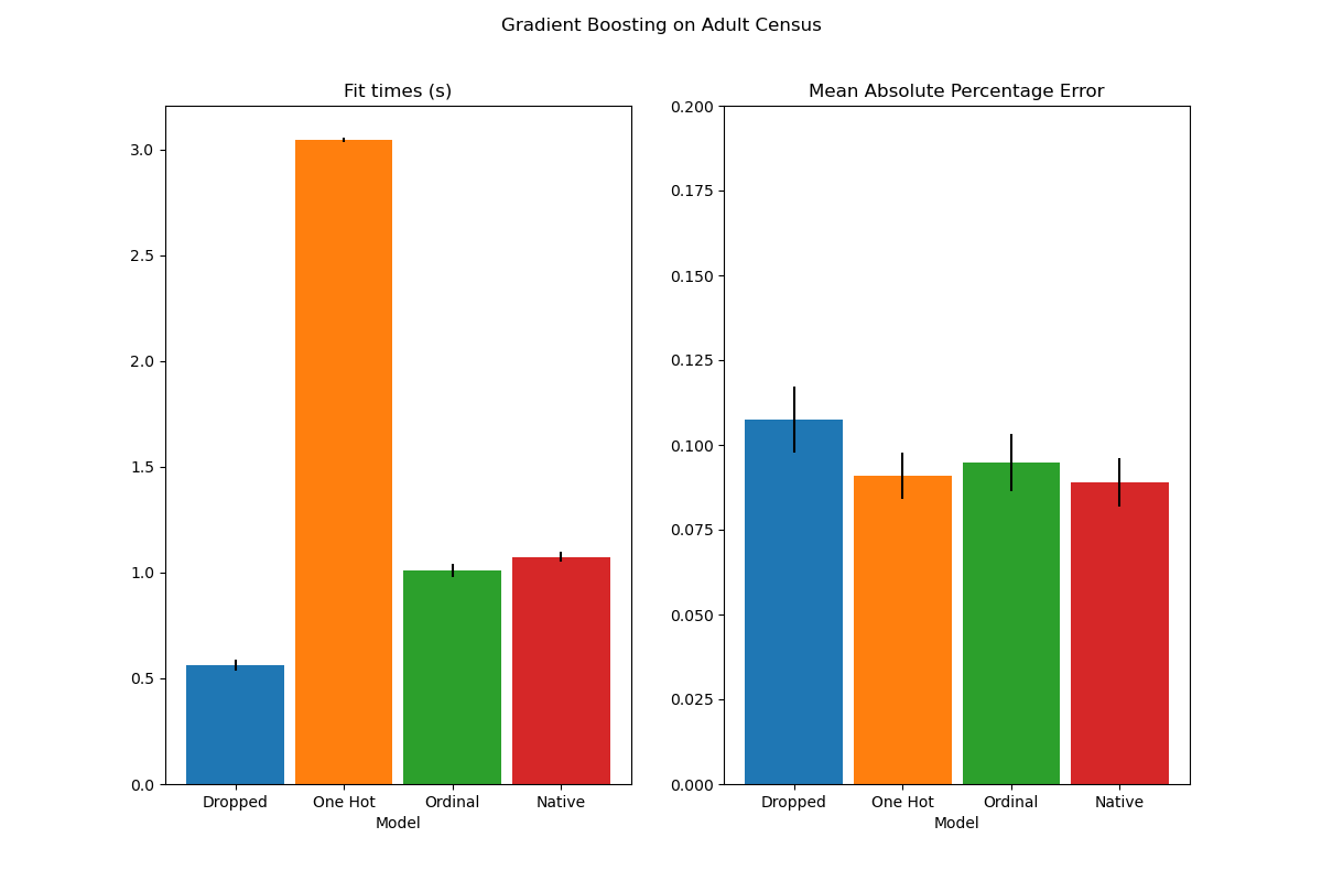
plot_results("Gradient Boosting on Adult Census")

We see that the model with one-hot-encoded data is by far the slowest. This is to be expected, since one-hot-encoding creates one additional feature per category value (for each categorical feature), and thus more split points need to be considered during fitting. In theory, we expect the native handling of categorical features to be slightly slower than treating categories as ordered quantities (‘Ordinal’), since native handling requires sorting categories. Fitting times should however be close when the number of categories is small, and this may not always be reflected in practice.

In terms of prediction performance, dropping the categorical features leads to poorer performance. The three models that use categorical features have comparable error rates, with a slight edge for the native handling.

Limitting the number of splits¶

In general, one can expect poorer predictions from one-hot-encoded data, especially when the tree depths or the number of nodes are limited: with one-hot-encoded data, one needs more split points, i.e. more depth, in order to recover an equivalent split that could be obtained in one single split point with native handling.

This is also true when categories are treated as ordinal quantities: if categories are A..F and the best split is ACF - BDE the one-hot-encoder model will need 3 split points (one per category in the left node), and the ordinal non-native model will need 4 splits: 1 split to isolate A, 1 split to isolate F, and 2 splits to isolate C from BCDE.

How strongly the models’ performances differ in practice will depend on the dataset and on the flexibility of the trees.

To see this, let us re-run the same analysis with under-fitting models where we artificially limit the total number of splits by both limitting the number of trees and the depth of each tree.

for pipe in (hist_dropped, hist_one_hot, hist_ordinal, hist_native):
    pipe.set_params(histgradientboostingregressor__max_depth=3,
                    histgradientboostingregressor__max_iter=15)

dropped_result = cross_validate(hist_dropped, X, y, cv=3, scoring=scoring)
one_hot_result = cross_validate(hist_one_hot, X, y, cv=3, scoring=scoring)
ordinal_result = cross_validate(hist_ordinal, X, y, cv=3, scoring=scoring)
native_result = cross_validate(hist_native, X, y, cv=3, scoring=scoring)

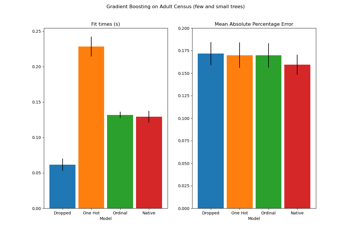
plot_results("Gradient Boosting on Adult Census (few and small trees)")

plt.show()

The results for these under-fitting models confirm our previous intuition: the native category handling strategy performs the best when the splitting budget is constrained. The two other strategies (one-hot encoding and treating categories as ordinal values) lead to error values comparable to the baseline model that just dropped the categorical features altogether.

Total running time of the script: ( 0 minutes 22.461 seconds)

Download Python source code: plot_gradient_boosting_categorical.py

Download Jupyter notebook: plot_gradient_boosting_categorical.ipynb

Gallery generated by Sphinx-Gallery