Note
Click here to download the full example code or to run this example in your browser via Binder
A demo of K-Means clustering on the handwritten digits data
In this example we compare the various initialization strategies for K-means in terms of runtime and quality of the results.
As the ground truth is known here, we also apply different cluster quality metrics to judge the goodness of fit of the cluster labels to the ground truth.
Cluster quality metrics evaluated (see Clustering performance evaluation for definitions and discussions of the metrics):
Shorthand |
full name |
|---|---|
homo |
homogeneity score |
compl |
completeness score |
v-meas |
V measure |
ARI |
adjusted Rand index |
AMI |
adjusted mutual information |
silhouette |
silhouette coefficient |
print(__doc__)
Load the dataset
We will start by loading the digits dataset. This dataset contains
handwritten digits from 0 to 9. In the context of clustering, one would like
to group images such that the handwritten digits on the image are the same.
import numpy as np
from sklearn.datasets import load_digits

data, labels = load_digits(return_X_y=True)
(n_samples, n_features), n_digits = data.shape, np.unique(labels).size

print(
    f"# digits: {n_digits}; # samples: {n_samples}; # features {n_features}"
)
Out:
# digits: 10; # samples: 1797; # features 64
Define our evaluation benchmark
We will first our evaluation benchmark. During this benchmark, we intend to compare different initialization methods for KMeans. Our benchmark will:
create a pipeline which will scale the data using a
StandardScaler;train and time the pipeline fitting;
measure the performance of the clustering obtained via different metrics.
from time import time
from sklearn import metrics
from sklearn.pipeline import make_pipeline
from sklearn.preprocessing import StandardScaler


def bench_k_means(kmeans, name, data, labels):
    """Benchmark to evaluate the KMeans initialization methods.

    Parameters
    ----------
    kmeans : KMeans instance
        A :class:`~sklearn.cluster.KMeans` instance with the initialization
        already set.
    name : str
        Name given to the strategy. It will be used to show the results in a
        table.
    data : ndarray of shape (n_samples, n_features)
        The data to cluster.
    labels : ndarray of shape (n_samples,)
        The labels used to compute the clustering metrics which requires some
        supervision.
    """
    t0 = time()
    estimator = make_pipeline(StandardScaler(), kmeans).fit(data)
    fit_time = time() - t0
    results = [name, fit_time, estimator[-1].inertia_]

    # Define the metrics which require only the true labels and estimator
    # labels
    clustering_metrics = [
        metrics.homogeneity_score,
        metrics.completeness_score,
        metrics.v_measure_score,
        metrics.adjusted_rand_score,
        metrics.adjusted_mutual_info_score,
    ]
    results += [m(labels, estimator[-1].labels_) for m in clustering_metrics]

    # The silhouette score requires the full dataset
    results += [
        metrics.silhouette_score(data, estimator[-1].labels_,
                                 metric="euclidean", sample_size=300,)
    ]

    # Show the results
    formatter_result = ("{:9s}\t{:.3f}s\t{:.0f}\t{:.3f}\t{:.3f}"
                        "\t{:.3f}\t{:.3f}\t{:.3f}\t{:.3f}")
    print(formatter_result.format(*results))
Run the benchmark
We will compare three approaches:
an initialization using
kmeans++. This method is stochastic and we will run the initialization 4 times;a random initialization. This method is stochastic as well and we will run the initialization 4 times;
an initialization based on a
PCAprojection. Indeed, we will use the components of thePCAto initialize KMeans. This method is deterministic and a single initialization suffice.
from sklearn.cluster import KMeans
from sklearn.decomposition import PCA

print(82 * '_')
print('init\t\ttime\tinertia\thomo\tcompl\tv-meas\tARI\tAMI\tsilhouette')

kmeans = KMeans(init="k-means++", n_clusters=n_digits, n_init=4,
                random_state=0)
bench_k_means(kmeans=kmeans, name="k-means++", data=data, labels=labels)

kmeans = KMeans(init="random", n_clusters=n_digits, n_init=4, random_state=0)
bench_k_means(kmeans=kmeans, name="random", data=data, labels=labels)

pca = PCA(n_components=n_digits).fit(data)
kmeans = KMeans(init=pca.components_, n_clusters=n_digits, n_init=1)
bench_k_means(kmeans=kmeans, name="PCA-based", data=data, labels=labels)

print(82 * '_')
Out:
__________________________________________________________________________________
init            time    inertia homo    compl   v-meas  ARI     AMI     silhouette
k-means++       0.091s  69662   0.680   0.719   0.699   0.570   0.695   0.173
random          0.055s  69707   0.675   0.716   0.694   0.560   0.691   0.188
PCA-based       0.039s  72686   0.636   0.658   0.647   0.521   0.643   0.144
__________________________________________________________________________________
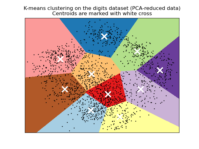
Visualize the results on PCA-reduced data
PCA allows to project the data from the
original 64-dimensional space into a lower dimensional space. Subsequently,
we can use PCA to project into a
2-dimensional space and plot the data and the clusters in this new space.
import matplotlib.pyplot as plt

reduced_data = PCA(n_components=2).fit_transform(data)
kmeans = KMeans(init="k-means++", n_clusters=n_digits, n_init=4)
kmeans.fit(reduced_data)

# Step size of the mesh. Decrease to increase the quality of the VQ.
h = .02     # point in the mesh [x_min, x_max]x[y_min, y_max].

# Plot the decision boundary. For that, we will assign a color to each
x_min, x_max = reduced_data[:, 0].min() - 1, reduced_data[:, 0].max() + 1
y_min, y_max = reduced_data[:, 1].min() - 1, reduced_data[:, 1].max() + 1
xx, yy = np.meshgrid(np.arange(x_min, x_max, h), np.arange(y_min, y_max, h))

# Obtain labels for each point in mesh. Use last trained model.
Z = kmeans.predict(np.c_[xx.ravel(), yy.ravel()])

# Put the result into a color plot
Z = Z.reshape(xx.shape)
plt.figure(1)
plt.clf()
plt.imshow(Z, interpolation="nearest",
           extent=(xx.min(), xx.max(), yy.min(), yy.max()),
           cmap=plt.cm.Paired, aspect="auto", origin="lower")

plt.plot(reduced_data[:, 0], reduced_data[:, 1], 'k.', markersize=2)
# Plot the centroids as a white X
centroids = kmeans.cluster_centers_
plt.scatter(centroids[:, 0], centroids[:, 1], marker="x", s=169, linewidths=3,
            color="w", zorder=10)
plt.title("K-means clustering on the digits dataset (PCA-reduced data)\n"
          "Centroids are marked with white cross")
plt.xlim(x_min, x_max)
plt.ylim(y_min, y_max)
plt.xticks(())
plt.yticks(())
plt.show()
Total running time of the script: ( 0 minutes 1.099 seconds)