Note
Click here to download the full example code or to run this example in your browser via Binder
Recognizing hand-written digits
This example shows how scikit-learn can be used to recognize images of hand-written digits, from 0-9.
print(__doc__)

# Author: Gael Varoquaux <gael dot varoquaux at normalesup dot org>
# License: BSD 3 clause

# Standard scientific Python imports
import matplotlib.pyplot as plt

# Import datasets, classifiers and performance metrics
from sklearn import datasets, svm, metrics
from sklearn.model_selection import train_test_split
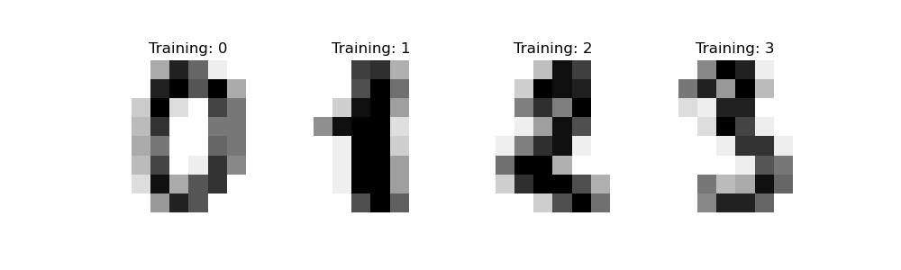
Digits dataset
The digits dataset consists of 8x8
pixel images of digits. The images attribute of the dataset stores
8x8 arrays of grayscale values for each image. We will use these arrays to
visualize the first 4 images. The target attribute of the dataset stores
the digit each image represents and this is included in the title of the 4
plots below.
Note: if we were working from image files (e.g., ‘png’ files), we would load
them using matplotlib.pyplot.imread.
digits = datasets.load_digits()

_, axes = plt.subplots(nrows=1, ncols=4, figsize=(10, 3))
for ax, image, label in zip(axes, digits.images, digits.target):
    ax.set_axis_off()
    ax.imshow(image, cmap=plt.cm.gray_r, interpolation='nearest')
    ax.set_title('Training: %i' % label)
Classification
To apply a classifier on this data, we need to flatten the images, turning
each 2-D array of grayscale values from shape (8, 8) into shape
(64,). Subsequently, the entire dataset will be of shape
(n_samples, n_features), where n_samples is the number of images and
n_features is the total number of pixels in each image.
We can then split the data into train and test subsets and fit a support vector classifier on the train samples. The fitted classifier can subsequently be used to predict the value of the digit for the samples in the test subset.
# flatten the images
n_samples = len(digits.images)
data = digits.images.reshape((n_samples, -1))

# Create a classifier: a support vector classifier
clf = svm.SVC(gamma=0.001)

# Split data into 50% train and 50% test subsets
X_train, X_test, y_train, y_test = train_test_split(
    data, digits.target, test_size=0.5, shuffle=False)

# Learn the digits on the train subset
clf.fit(X_train, y_train)

# Predict the value of the digit on the test subset
predicted = clf.predict(X_test)
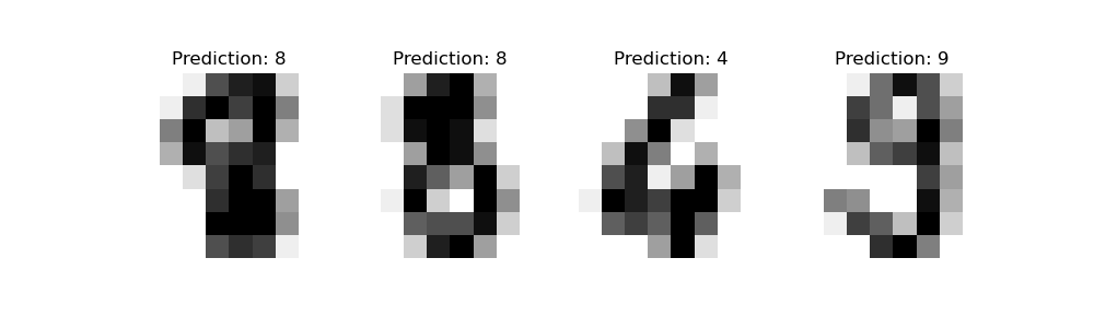
Below we visualize the first 4 test samples and show their predicted digit value in the title.
_, axes = plt.subplots(nrows=1, ncols=4, figsize=(10, 3))
for ax, image, prediction in zip(axes, X_test, predicted):
    ax.set_axis_off()
    image = image.reshape(8, 8)
    ax.imshow(image, cmap=plt.cm.gray_r, interpolation='nearest')
    ax.set_title(f'Prediction: {prediction}')
classification_report builds a text report showing
the main classification metrics.
print(f"Classification report for classifier {clf}:\n"
      f"{metrics.classification_report(y_test, predicted)}\n")
Out:
Classification report for classifier SVC(gamma=0.001):
              precision    recall  f1-score   support

           0       1.00      0.99      0.99        88
           1       0.99      0.97      0.98        91
           2       0.99      0.99      0.99        86
           3       0.98      0.87      0.92        91
           4       0.99      0.96      0.97        92
           5       0.95      0.97      0.96        91
           6       0.99      0.99      0.99        91
           7       0.96      0.99      0.97        89
           8       0.94      1.00      0.97        88
           9       0.93      0.98      0.95        92

    accuracy                           0.97       899
   macro avg       0.97      0.97      0.97       899
weighted avg       0.97      0.97      0.97       899
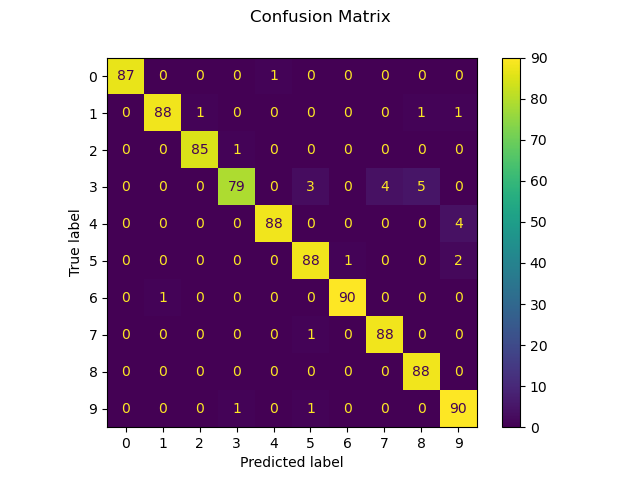
We can also plot a confusion matrix of the true digit values and the predicted digit values.
disp = metrics.plot_confusion_matrix(clf, X_test, y_test)
disp.figure_.suptitle("Confusion Matrix")
print(f"Confusion matrix:\n{disp.confusion_matrix}")

plt.show()
Out:
Confusion matrix:
[[87  0  0  0  1  0  0  0  0  0]
 [ 0 88  1  0  0  0  0  0  1  1]
 [ 0  0 85  1  0  0  0  0  0  0]
 [ 0  0  0 79  0  3  0  4  5  0]
 [ 0  0  0  0 88  0  0  0  0  4]
 [ 0  0  0  0  0 88  1  0  0  2]
 [ 0  1  0  0  0  0 90  0  0  0]
 [ 0  0  0  0  0  1  0 88  0  0]
 [ 0  0  0  0  0  0  0  0 88  0]
 [ 0  0  0  1  0  1  0  0  0 90]]
Total running time of the script: ( 0 minutes 0.795 seconds)