Note
Click here to download the full example code or to run this example in your browser via Binder
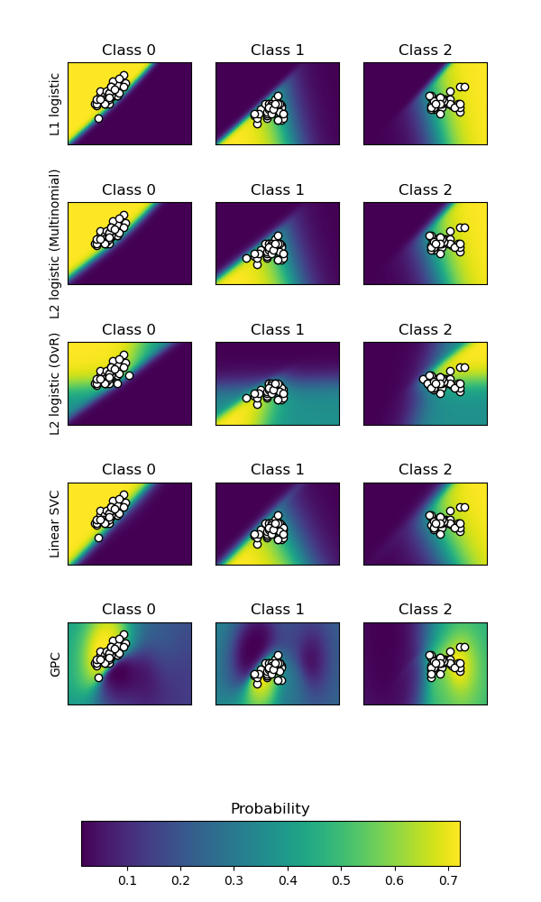
Plot classification probability
Plot the classification probability for different classifiers. We use a 3 class dataset, and we classify it with a Support Vector classifier, L1 and L2 penalized logistic regression with either a One-Vs-Rest or multinomial setting, and Gaussian process classification.
Linear SVC is not a probabilistic classifier by default but it has a built-in
calibration option enabled in this example (probability=True).
The logistic regression with One-Vs-Rest is not a multiclass classifier out of the box. As a result it has more trouble in separating class 2 and 3 than the other estimators.
Out:
Accuracy (train) for L1 logistic: 83.3%
Accuracy (train) for L2 logistic (Multinomial): 82.7%
Accuracy (train) for L2 logistic (OvR): 79.3%
Accuracy (train) for Linear SVC: 82.0%
Accuracy (train) for GPC: 82.7%
print(__doc__)

# Author: Alexandre Gramfort <alexandre.gramfort@inria.fr>
# License: BSD 3 clause

import matplotlib.pyplot as plt
import numpy as np

from sklearn.metrics import accuracy_score
from sklearn.linear_model import LogisticRegression
from sklearn.svm import SVC
from sklearn.gaussian_process import GaussianProcessClassifier
from sklearn.gaussian_process.kernels import RBF
from sklearn import datasets

iris = datasets.load_iris()
X = iris.data[:, 0:2]  # we only take the first two features for visualization
y = iris.target

n_features = X.shape[1]

C = 10
kernel = 1.0 * RBF([1.0, 1.0])  # for GPC

# Create different classifiers.
classifiers = {
    'L1 logistic': LogisticRegression(C=C, penalty='l1',
                                      solver='saga',
                                      multi_class='multinomial',
                                      max_iter=10000),
    'L2 logistic (Multinomial)': LogisticRegression(C=C, penalty='l2',
                                                    solver='saga',
                                                    multi_class='multinomial',
                                                    max_iter=10000),
    'L2 logistic (OvR)': LogisticRegression(C=C, penalty='l2',
                                            solver='saga',
                                            multi_class='ovr',
                                            max_iter=10000),
    'Linear SVC': SVC(kernel='linear', C=C, probability=True,
                      random_state=0),
    'GPC': GaussianProcessClassifier(kernel)
}

n_classifiers = len(classifiers)

plt.figure(figsize=(3 * 2, n_classifiers * 2))
plt.subplots_adjust(bottom=.2, top=.95)

xx = np.linspace(3, 9, 100)
yy = np.linspace(1, 5, 100).T
xx, yy = np.meshgrid(xx, yy)
Xfull = np.c_[xx.ravel(), yy.ravel()]

for index, (name, classifier) in enumerate(classifiers.items()):
    classifier.fit(X, y)

    y_pred = classifier.predict(X)
    accuracy = accuracy_score(y, y_pred)
    print("Accuracy (train) for %s: %0.1f%% " % (name, accuracy * 100))

    # View probabilities:
    probas = classifier.predict_proba(Xfull)
    n_classes = np.unique(y_pred).size
    for k in range(n_classes):
        plt.subplot(n_classifiers, n_classes, index * n_classes + k + 1)
        plt.title("Class %d" % k)
        if k == 0:
            plt.ylabel(name)
        imshow_handle = plt.imshow(probas[:, k].reshape((100, 100)),
                                   extent=(3, 9, 1, 5), origin='lower')
        plt.xticks(())
        plt.yticks(())
        idx = (y_pred == k)
        if idx.any():
            plt.scatter(X[idx, 0], X[idx, 1], marker='o', c='w', edgecolor='k')

ax = plt.axes([0.15, 0.04, 0.7, 0.05])
plt.title("Probability")
plt.colorbar(imshow_handle, cax=ax, orientation='horizontal')

plt.show()
Total running time of the script: ( 0 minutes 1.454 seconds)