Note

Click here to download the full example code or to run this example in your browser via Binder

Combine predictors using stacking¶

Stacking refers to a method to blend estimators. In this strategy, some estimators are individually fitted on some training data while a final estimator is trained using the stacked predictions of these base estimators.

In this example, we illustrate the use case in which different regressors are stacked together and a final linear penalized regressor is used to output the prediction. We compare the performance of each individual regressor with the stacking strategy. Stacking slightly improves the overall performance.

print(__doc__)

# Authors: Guillaume Lemaitre <g.lemaitre58@gmail.com>
#          Maria Telenczuk    <https://github.com/maikia>
# License: BSD 3 clause

Download the dataset¶

We will use Ames Housing dataset which was first compiled by Dean De Cock and became better known after it was used in Kaggle challenge. It is a set of 1460 residential homes in Ames, Iowa, each described by 80 features. We will use it to predict the final logarithmic price of the houses. In this example we will use only 20 most interesting features chosen using GradientBoostingRegressor() and limit number of entries (here we won’t go into the details on how to select the most interesting features).

The Ames housing dataset is not shipped with scikit-learn and therefore we will fetch it from OpenML.

import numpy as np

from sklearn.datasets import fetch_openml
from sklearn.utils import shuffle


def load_ames_housing():
    df = fetch_openml(name="house_prices", as_frame=True)
    X = df.data
    y = df.target

    features = ['YrSold', 'HeatingQC', 'Street', 'YearRemodAdd', 'Heating',
                'MasVnrType', 'BsmtUnfSF', 'Foundation', 'MasVnrArea',
                'MSSubClass', 'ExterQual', 'Condition2', 'GarageCars',
                'GarageType', 'OverallQual', 'TotalBsmtSF', 'BsmtFinSF1',
                'HouseStyle', 'MiscFeature', 'MoSold']

    X = X[features]
    X, y = shuffle(X, y, random_state=0)

    X = X[:600]
    y = y[:600]
    return X, np.log(y)


X, y = load_ames_housing()

Make pipeline to preprocess the data¶

Before we can use Ames dataset we still need to do some preprocessing. First, the dataset has many missing values. To impute them, we will exchange categorical missing values with the new category ‘missing’ while the numerical missing values with the ‘mean’ of the column. We will also encode the categories with either sklearn.preprocessing.OneHotEncoder or sklearn.preprocessing.OrdinalEncoder depending for which type of model we will use them (linear or non-linear model). To falicitate this preprocessing we will make two pipelines. You can skip this section if your data is ready to use and does not need preprocessing

from sklearn.compose import make_column_transformer
from sklearn.impute import SimpleImputer
from sklearn.pipeline import make_pipeline
from sklearn.preprocessing import OneHotEncoder
from sklearn.preprocessing import OrdinalEncoder
from sklearn.preprocessing import StandardScaler


cat_cols = X.columns[X.dtypes == 'O']
num_cols = X.columns[X.dtypes == 'float64']

categories = [
    X[column].unique() for column in X[cat_cols]]

for cat in categories:
    cat[cat == None] = 'missing'  # noqa

cat_proc_nlin = make_pipeline(
    SimpleImputer(missing_values=None, strategy='constant',
                  fill_value='missing'),
    OrdinalEncoder(categories=categories)
    )

num_proc_nlin = make_pipeline(SimpleImputer(strategy='mean'))

cat_proc_lin = make_pipeline(
    SimpleImputer(missing_values=None,
                  strategy='constant',
                  fill_value='missing'),
    OneHotEncoder(categories=categories)
)

num_proc_lin = make_pipeline(
    SimpleImputer(strategy='mean'),
    StandardScaler()
)

# transformation to use for non-linear estimators
processor_nlin = make_column_transformer(
    (cat_proc_nlin, cat_cols),
    (num_proc_nlin, num_cols),
    remainder='passthrough')

# transformation to use for linear estimators
processor_lin = make_column_transformer(
    (cat_proc_lin, cat_cols),
    (num_proc_lin, num_cols),
    remainder='passthrough')

Stack of predictors on a single data set¶

It is sometimes tedious to find the model which will best perform on a given dataset. Stacking provide an alternative by combining the outputs of several learners, without the need to choose a model specifically. The performance of stacking is usually close to the best model and sometimes it can outperform the prediction performance of each individual model.

Here, we combine 3 learners (linear and non-linear) and use a ridge regressor to combine their outputs together.

Note: although we will make new pipelines with the processors which we wrote in the previous section for the 3 learners, the final estimator RidgeCV() does not need preprocessing of the data as it will be fed with the already preprocessed output from the 3 learners.

from sklearn.experimental import enable_hist_gradient_boosting  # noqa
from sklearn.ensemble import HistGradientBoostingRegressor
from sklearn.ensemble import RandomForestRegressor
from sklearn.ensemble import StackingRegressor
from sklearn.linear_model import LassoCV
from sklearn.linear_model import RidgeCV


lasso_pipeline = make_pipeline(processor_lin,
                               LassoCV())

rf_pipeline = make_pipeline(processor_nlin,
                            RandomForestRegressor(random_state=42))

gradient_pipeline = make_pipeline(
    processor_nlin,
    HistGradientBoostingRegressor(random_state=0))

estimators = [('Random Forest', rf_pipeline),
              ('Lasso', lasso_pipeline),
              ('Gradient Boosting', gradient_pipeline)]

stacking_regressor = StackingRegressor(estimators=estimators,
                                       final_estimator=RidgeCV())

Measure and plot the results¶

Now we can use Ames Housing dataset to make the predictions. We check the performance of each individual predictor as well as of the stack of the regressors.

The function plot_regression_results is used to plot the predicted and true targets.

import time
import matplotlib.pyplot as plt
from sklearn.model_selection import cross_validate, cross_val_predict


def plot_regression_results(ax, y_true, y_pred, title, scores, elapsed_time):
    """Scatter plot of the predicted vs true targets."""
    ax.plot([y_true.min(), y_true.max()],
            [y_true.min(), y_true.max()],
            '--r', linewidth=2)
    ax.scatter(y_true, y_pred, alpha=0.2)

    ax.spines['top'].set_visible(False)
    ax.spines['right'].set_visible(False)
    ax.get_xaxis().tick_bottom()
    ax.get_yaxis().tick_left()
    ax.spines['left'].set_position(('outward', 10))
    ax.spines['bottom'].set_position(('outward', 10))
    ax.set_xlim([y_true.min(), y_true.max()])
    ax.set_ylim([y_true.min(), y_true.max()])
    ax.set_xlabel('Measured')
    ax.set_ylabel('Predicted')
    extra = plt.Rectangle((0, 0), 0, 0, fc="w", fill=False,
                          edgecolor='none', linewidth=0)
    ax.legend([extra], [scores], loc='upper left')
    title = title + '\n Evaluation in {:.2f} seconds'.format(elapsed_time)
    ax.set_title(title)


fig, axs = plt.subplots(2, 2, figsize=(9, 7))
axs = np.ravel(axs)

for ax, (name, est) in zip(axs, estimators + [('Stacking Regressor',
                                               stacking_regressor)]):
    start_time = time.time()
    score = cross_validate(est, X, y,
                           scoring=['r2', 'neg_mean_absolute_error'],
                           n_jobs=-1, verbose=0)
    elapsed_time = time.time() - start_time

    y_pred = cross_val_predict(est, X, y, n_jobs=-1, verbose=0)

    plot_regression_results(
        ax, y, y_pred,
        name,
        (r'$R^2={:.2f} \pm {:.2f}$' + '\n' + r'$MAE={:.2f} \pm {:.2f}$')
        .format(np.mean(score['test_r2']),
                np.std(score['test_r2']),
                -np.mean(score['test_neg_mean_absolute_error']),
                np.std(score['test_neg_mean_absolute_error'])),
        elapsed_time)

plt.suptitle('Single predictors versus stacked predictors')
plt.tight_layout()
plt.subplots_adjust(top=0.9)
plt.show()

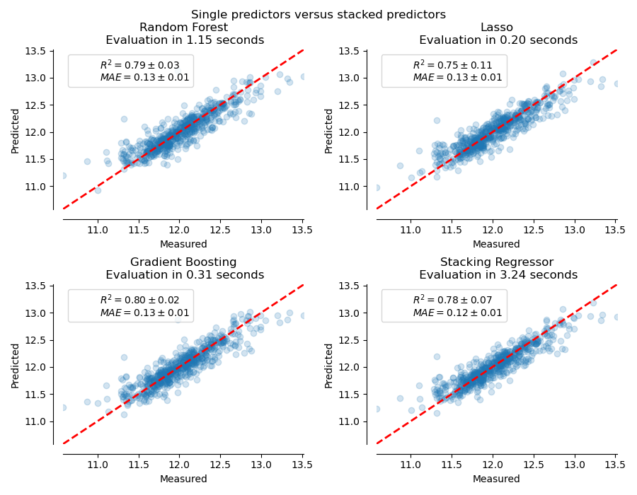
Single predictors versus stacked predictors, Random Forest Evaluation in 1.15 seconds, Lasso Evaluation in 0.20 seconds, Gradient Boosting Evaluation in 0.31 seconds, Stacking Regressor Evaluation in 3.24 seconds

The stacked regressor will combine the strengths of the different regressors. However, we also see that training the stacked regressor is much more computationally expensive.

Total running time of the script: ( 0 minutes 10.681 seconds)

Gallery generated by Sphinx-Gallery