Note
Click here to download the full example code or to run this example in your browser via Binder
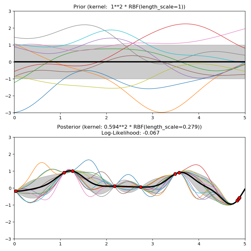
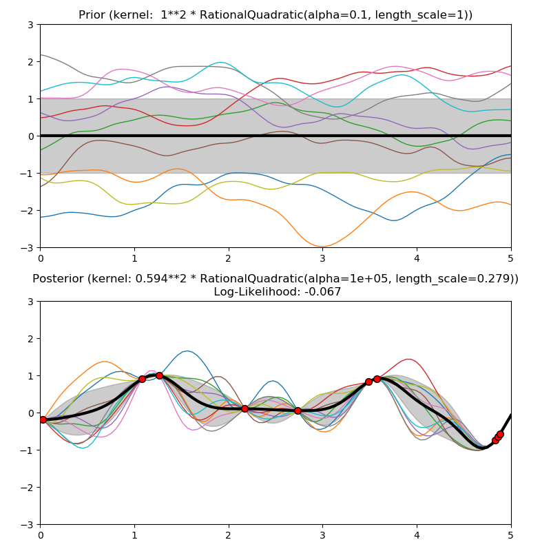
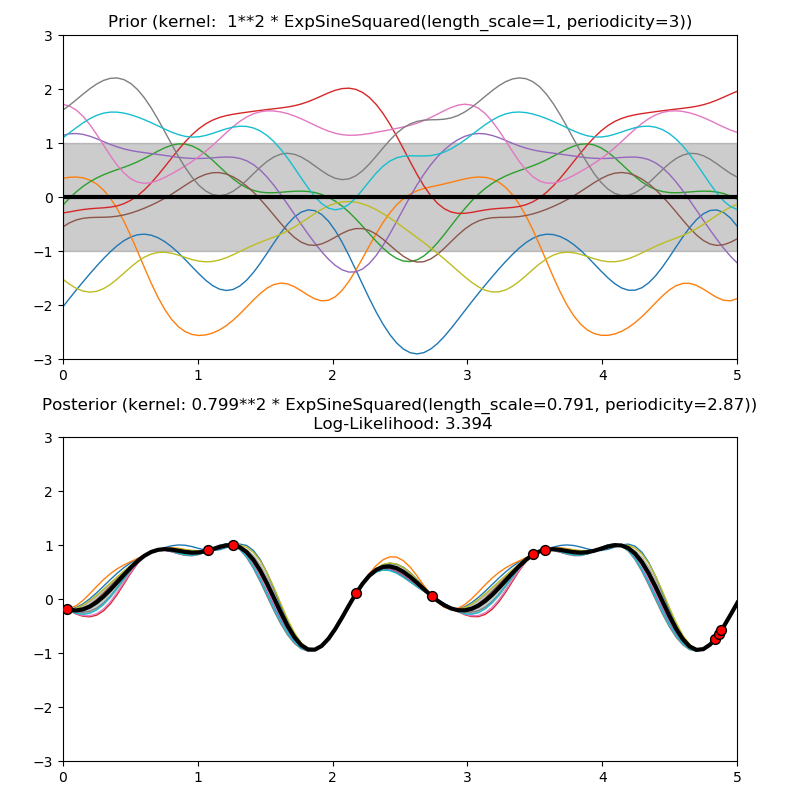
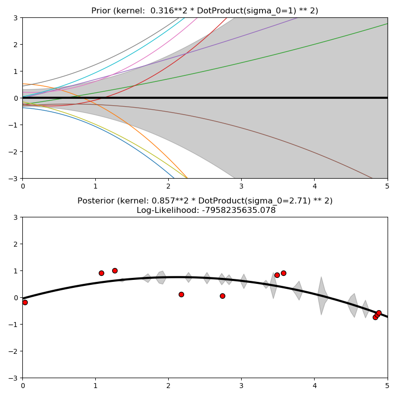
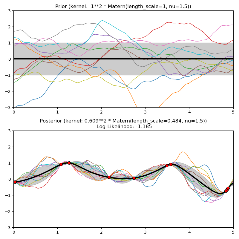
Illustration of prior and posterior Gaussian process for different kernels
This example illustrates the prior and posterior of a GPR with different kernels. Mean, standard deviation, and 10 samples are shown for both prior and posterior.
Out:
/home/circleci/project/sklearn/gaussian_process/_gpr.py:494: ConvergenceWarning: lbfgs failed to converge (status=2):
ABNORMAL_TERMINATION_IN_LNSRCH.

Increase the number of iterations (max_iter) or scale the data as shown in:
    https://scikit-learn.org/stable/modules/preprocessing.html
  _check_optimize_result("lbfgs", opt_res)
/home/circleci/project/sklearn/gaussian_process/_gpr.py:362: UserWarning: Predicted variances smaller than 0. Setting those variances to 0.
  warnings.warn("Predicted variances smaller than 0. "
print(__doc__)

# Authors: Jan Hendrik Metzen <jhm@informatik.uni-bremen.de>
#
# License: BSD 3 clause

import numpy as np

from matplotlib import pyplot as plt

from sklearn.gaussian_process import GaussianProcessRegressor
from sklearn.gaussian_process.kernels import (RBF, Matern, RationalQuadratic,
                                              ExpSineSquared, DotProduct,
                                              ConstantKernel)


kernels = [1.0 * RBF(length_scale=1.0, length_scale_bounds=(1e-1, 10.0)),
           1.0 * RationalQuadratic(length_scale=1.0, alpha=0.1),
           1.0 * ExpSineSquared(length_scale=1.0, periodicity=3.0,
                                length_scale_bounds=(0.1, 10.0),
                                periodicity_bounds=(1.0, 10.0)),
           ConstantKernel(0.1, (0.01, 10.0))
               * (DotProduct(sigma_0=1.0, sigma_0_bounds=(0.1, 10.0)) ** 2),
           1.0 * Matern(length_scale=1.0, length_scale_bounds=(1e-1, 10.0),
                        nu=1.5)]

for kernel in kernels:
    # Specify Gaussian Process
    gp = GaussianProcessRegressor(kernel=kernel)

    # Plot prior
    plt.figure(figsize=(8, 8))
    plt.subplot(2, 1, 1)
    X_ = np.linspace(0, 5, 100)
    y_mean, y_std = gp.predict(X_[:, np.newaxis], return_std=True)
    plt.plot(X_, y_mean, 'k', lw=3, zorder=9)
    plt.fill_between(X_, y_mean - y_std, y_mean + y_std,
                     alpha=0.2, color='k')
    y_samples = gp.sample_y(X_[:, np.newaxis], 10)
    plt.plot(X_, y_samples, lw=1)
    plt.xlim(0, 5)
    plt.ylim(-3, 3)
    plt.title("Prior (kernel:  %s)" % kernel, fontsize=12)

    # Generate data and fit GP
    rng = np.random.RandomState(4)
    X = rng.uniform(0, 5, 10)[:, np.newaxis]
    y = np.sin((X[:, 0] - 2.5) ** 2)
    gp.fit(X, y)

    # Plot posterior
    plt.subplot(2, 1, 2)
    X_ = np.linspace(0, 5, 100)
    y_mean, y_std = gp.predict(X_[:, np.newaxis], return_std=True)
    plt.plot(X_, y_mean, 'k', lw=3, zorder=9)
    plt.fill_between(X_, y_mean - y_std, y_mean + y_std,
                     alpha=0.2, color='k')

    y_samples = gp.sample_y(X_[:, np.newaxis], 10)
    plt.plot(X_, y_samples, lw=1)
    plt.scatter(X[:, 0], y, c='r', s=50, zorder=10, edgecolors=(0, 0, 0))
    plt.xlim(0, 5)
    plt.ylim(-3, 3)
    plt.title("Posterior (kernel: %s)\n Log-Likelihood: %.3f"
              % (gp.kernel_, gp.log_marginal_likelihood(gp.kernel_.theta)),
              fontsize=12)
    plt.tight_layout()

plt.show()
Total running time of the script: ( 0 minutes 1.239 seconds)
Estimated memory usage: 8 MB