
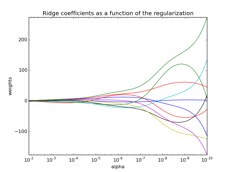
Plot Ridge coefficients as a function of the regularization
Shows the effect of collinearity in the coefficients of an estimator.
Ridge Regression is the estimator used in this example. Each color represents a different feature of the coefficient vector, and this is displayed as a function of the regularization parameter.
At the end of the path, as alpha tends toward zero and the solution tends towards the ordinary least squares, coefficients exhibit big oscillations.
Python source code: plot_ridge_path.py
# Author: Fabian Pedregosa -- <fabian.pedregosa@inria.fr>
# License: BSD 3 clause

print(__doc__)

import numpy as np
import matplotlib.pyplot as plt
from sklearn import linear_model

# X is the 10x10 Hilbert matrix
X = 1. / (np.arange(1, 11) + np.arange(0, 10)[:, np.newaxis])
y = np.ones(10)

###############################################################################
# Compute paths

n_alphas = 200
alphas = np.logspace(-10, -2, n_alphas)
clf = linear_model.Ridge(fit_intercept=False)

coefs = []
for a in alphas:
    clf.set_params(alpha=a)
    clf.fit(X, y)
    coefs.append(clf.coef_)

###############################################################################
# Display results

ax = plt.gca()
ax.set_color_cycle(['b', 'r', 'g', 'c', 'k', 'y', 'm'])

ax.plot(alphas, coefs)
ax.set_xscale('log')
ax.set_xlim(ax.get_xlim()[::-1])  # reverse axis
plt.xlabel('alpha')
plt.ylabel('weights')
plt.title('Ridge coefficients as a function of the regularization')
plt.axis('tight')
plt.show()
Total running time of the example: 0.13 seconds ( 0 minutes 0.13 seconds)